This post is a work in progress and may be updated or expanded soon!

Basics

Camera Transformations

To map a 3D world point to the image, we use two steps:

1. Convert the point from world coordinates to camera coordinates.
2. Project the camera-space point to pixel coordinates using the intrinsics.

---

1. World $\rightarrow$ Camera Coordinates

Let the camera center be $C$ and orientation be $R$.
A world point $X$ is mapped into camera coordinates by

$$ X_C = R(X - C). $$

Define the translation

$$ t = -RC, $$

so the extrinsic mapping becomes

$$ X_C = RX + t. $$

In homogeneous coordinates:

$$ \begin{bmatrix} X_C \\ Y_C \\ Z_C \\ 1 \end{bmatrix}=\begin{bmatrix} R & t \\ 0 & 1 \end{bmatrix} \begin{bmatrix} X \\ Y \\ Z \\ 1 \end{bmatrix}. $$

---

2. Camera $\rightarrow$ Pixel Coordinates

A point in the camera frame projects via

$$ u = \frac{X_C}{Z_C}, \qquad v = \frac{Y_C}{Z_C}. $$

To convert into pixels, we apply the intrinsic matrix

$$ K = \begin{bmatrix} f_x & 0 & c_x \\ 0 & f_y & c_y \\ 0 & 0 & 1 \end{bmatrix}. $$

This gives

$$ u = \frac{f_x X_C}{Z_C} + c_x, \qquad v = \frac{f_y Y_C}{Z_C} + c_y. $$

Combined:

$$ \begin{bmatrix}u \\ v \\ 1\end{bmatrix}= K\,[R\;t] \begin{bmatrix}X \\ Y \\ Z \\ 1\end{bmatrix}, \qquad s = Z_C. $$

---

3. Pixel $\rightarrow$ Camera Ray (Back-Projection)

To go from pixel $(u, v)$ back into camera space, we recover the ray direction.

Step 1: Remove intrinsics

$$ \begin{bmatrix} x \\ y \\ 1 \end{bmatrix}= K^{-1} \begin{bmatrix} u \\ v \\ 1 \end{bmatrix}. $$

Explicitly:

$$ x = \frac{u - c_x}{f_x}, \qquad y = \frac{v - c_y}{f_y}. $$

This gives the direction in camera coordinates:

$$ d_C = \begin{bmatrix} x \\ y \\ 1 \end{bmatrix}. $$

Step 2: Form the 3D ray

All 3D points along that pixel’s ray in camera space are:

$$ X_C(\lambda) = \lambda \, d_C = \lambda \begin{bmatrix} x \\ y \\ 1 \end{bmatrix}, \qquad \lambda>0. $$

Here

• $\lambda$ controls the depth,
• $d_C$ is the ray direction in the camera frame,
• the camera center is at the origin in camera coordinates, so there is no position term.

This is the complete back-projection from pixel $\rightarrow$ ray in camera space.

---

Forward and Inverse Camera Projection Pipeline

Interactive World 2 Cam

---

Inverse Transform Sampling

Definition

Let $U \sim \mathrm{Unif}[0,1]$. We want to generate a random variable $X$ with CDF $F_X(x)$.
Assume $F_X$ is continuous and strictly increasing so that it has a well-defined inverse.

We look for a strictly monotone transformation

$$ T : [0,1] \to \mathbb{R}, $$

such that the transformed variable $T(U)$ has the same distribution as $X$:

$$ T(U) \overset{d}{=} X. $$

Compute the CDF of $T(U)$:

$$ F_X(x) = \Pr(X \le x) = \Pr(T(U) \le x) = \Pr(U \le T^{-1}(x)). $$

Because $U \sim \mathrm{Unif}[0,1]$,

$$ \Pr(U \le y) = y, \qquad 0 \le y \le 1. $$

Thus,

$$ F_X(x) = T^{-1}(x). $$

So $F_X$ is the inverse of $T$, which implies

$$ T(u) = F_X^{-1}(u), \qquad u \in [0,1]. $$

Therefore, the desired random variable $X$ can be generated by

$$ X = F_X^{-1}(U). $$

Interactive Simulation

---

SfM

MPI

Stereo Magnification

---

Volume Rendering

The Physics of Light Transport

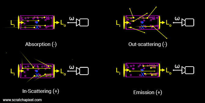
Unlike standard mesh rendering, where light bounces off a hard surface at a specific depth $z$, volume rendering assumes the scene is composed of particles that can emit and absorb light at any point in space (assuming no scattering of light).

The Differential Equation

Let a ray $\mathbf{r}(t) = \mathbf{o} + t\mathbf{d}$ travel through a volume. At any point $t$, the radiance (light energy) $L(t)$ changes based on two competing forces:

1. Absorption: The medium absorbs some existing light. The amount absorbed depends on the volume density $\sigma(t)$.
2. Emission: The medium adds new light (color) $\mathbf{c}(t)$, scaled by the density.

The change in radiance is described by the differential equation:

$$ \frac{d L(t)}{dt} = \underbrace{\sigma(t)\mathbf{c}(t)}_{\text{Gained Light}} - \underbrace{\sigma(t)L(t)}_{\text{Lost Light}} $$

The Integral Form

Solving this differential equation from the near plane $t_n$ to the far plane $t_f$ gives us the Volume Rendering Equation:

$$ C(\mathbf{r}) = \int_{t_n}^{t_f} T(t) \cdot \sigma(t) \cdot \mathbf{c}(t) \, dt $$

Where $T(t)$ is the Transmittance.

Intuition: Transmittance

Transmittance $T(t)$ represents the probability that a photon travels from the camera origin $t_n$ to the current point $t$ without being absorbed.

$$ T(t) = \exp\left( -\int_{t_n}^{t} \sigma(s) \, ds \right) $$

• If $\sigma(s) = 0$ everywhere (empty space), the integral is 0, and $T(t) = 1$ (perfect visibility).
• If $\sigma(s)$ is high (dense object), the integral becomes large, and $T(t) \to 0$ (occluded).

Proof

Consider what happens in an infinitesimal segment $[t, t + dt]$: - The probability of absorption in this segment is proportional to the density >$\sigma(t)$ and the distance $dt$ - The probability of absorption = $\sigma(t) \, dt$ - The probability of survival = $1 - \sigma(t) \, dt$

The Differential Equation

If $T(t)$ is the transmittance up to point $t$, then the transmittance at $t + dt$ is:

$$ T(t + dt) = T(t) \cdot (1 - \sigma(t) \, dt) $$

This says: “To survive to $t + dt$, you must survive to $t$ AND survive the next segment.”

Expanding:

$$ T(t + dt) = T(t) - T(t) \sigma(t) \, dt $$

Rearranging:

$$ T(t + dt) - T(t) = -T(t) \sigma(t) \, dt $$

Dividing both sides by $dt$:

$$ \frac{T(t + dt) - T(t)}{dt} = -T(t) \sigma(t) $$

Taking the limit as $dt \to 0$:

$$ \frac{dT(t)}{dt} = -\sigma(t) T(t) $$

Solving the ODE

This is a first-order separable differential equation. We separate variables:

$$ \frac{dT(t)}{T(t)} = -\sigma(t) \, dt $$

Integrate both sides from $t_n$ (starting point) to $t$ (current point):

$$ \int_{T(t_n)}^{T(t)} \frac{dT'}{T'} = -\int_{t_n}^{t} \sigma(s) \, ds $$

The left side evaluates to:

$$ \ln T(t) - \ln T(t_n) = -\int_{t_n}^{t} \sigma(s) \, ds $$$$ \ln \frac{T(t)}{T(t_n)} = -\int_{t_n}^{t} \sigma(s) \, ds $$

Initial Condition

At the ray origin ($t = t_n$), no absorption has occurred yet, so:

$$ T(t_n) = 1 $$

Substituting this:

$$ \ln T(t) = -\int_{t_n}^{t} \sigma(s) \, ds $$

Exponentiating both sides:

$$ T(t) = \exp\left( -\int_{t_n}^{t} \sigma(s) \, ds \right) $$

Special Cases:

• If $\sigma(s) = 0$ (vacuum): $T(t) = e^0 = 1$ (perfect transmission)
• If $\sigma(s) = \sigma_0$ (constant): $T(t) = e^{-\sigma_0 (t - t_n)}$ (exponential decay)
• As $\int \sigma(s) \, ds \to \infty$: $T(t) \to 0$ (complete occlusion)

In simple terms: The color of a pixel is the sum of all light emitted along the ray, weighted by how much “stuff” ($\sigma$) is at that point and how “clear” ($T$) the path is up to that point.

---

Discretization (Numerical Quadrature)

To estimate the above integral we must approximate it by breaking the ray into $N$ discrete segments (bins).

Let the ray be split into segments $[t_i, t_{i+1}]$. We assume the density $\sigma_i$ and color $\mathbf{c}_i$ are constant within each segment of length $\delta_i = t_{i+1} - t_i$.

1. From Density to Alpha ($\alpha$)

The probability that light is occluded within a single segment $i$ is given by standard exponential decay:

$$ \alpha_i = 1 - \exp(-\sigma_i \delta_i) $$

Here, $\alpha_i$ ranges from $[0, 1]$.

• $\sigma \to 0 \implies \alpha \to 0$ (Transparent)
• $\sigma \to \infty \implies \alpha \to 1$ (Opaque)

2. Discrete Transmittance

The transmittance $T_i$ (probability of reaching segment $i$) is the product of the “survival probabilities” of all previous segments:

$$ T_i = \prod_{j=1}^{i-1} (1 - \alpha_j) $$

3. The Compositing Formula

Substituting these into the integral gives the standard alpha-compositing formula used in NeRF, 3DGS, and traditional graphics:

$$ \hat{C}(\mathbf{r}) = \sum_{i=1}^{N} \underbrace{T_i}_{\text{Vis. to Cam}} \cdot \underbrace{\alpha_i}_{\text{Opacity}} \cdot \underbrace{\mathbf{c}_i}_{\text{Color}} $$

Or compactly, defining the contribution weight $w_i = T_i \alpha_i$:

$$ \hat{C}(\mathbf{r}) = \sum_{i=1}^{N} w_i \mathbf{c}_i $$

---

Proof: Summation of Weights

A common question is whether the weights $w_i = T_i \alpha_i$ sum to 1. This is crucial for treating the rendering process as an expectation.

Theorem: The sum of weights $\sum_{i=1}^N T_i \alpha_i$ equals $1 - T_{final}$. If the ray hits a fully opaque background (or extends infinitely into dense matter), the sum equals exactly 1.

Proof via Telescoping Sum:

Recall the definition of discrete transmittance:

$$ T_i = \prod_{j=1}^{i-1} (1 - \alpha_j) $$

The transmittance for the next step $T_{i+1}$ is:

$$ T_{i+1} = T_i (1 - \alpha_i) $$

We can rearrange this to solve for the weight term $T_i \alpha_i$:

$$ T_{i+1} = T_i - T_i \alpha_i $$

$$ T_i \alpha_i = T_i - T_{i+1} $$

Now, we sum this term over all samples $i=1$ to $N$:

$$ \sum_{i=1}^{N} w_i = \sum_{i=1}^{N} T_i \alpha_i = \sum_{i=1}^{N} (T_i - T_{i+1}) $$

This is a telescoping sum:

$$ \begin{aligned} \sum_{i=1}^{N} (T_i - T_{i+1}) &= (T_1 - T_2) \\ &+ (T_2 - T_3) \\ &+ \dots \\ &+ (T_N - T_{N+1}) \end{aligned} $$

Intermediate terms cancel out, leaving only the first and last terms:

$$ \sum_{i=1}^{N} w_i = T_1 - T_{N+1} $$

Since transmittance at the start of the ray (camera origin) is perfect visibility, $T_1 = 1$.

$$ \sum_{i=1}^{N} w_i = 1 - T_{N+1} $$

Conclusion: The weights sum to exactly 1 if and only if the remaining transmittance $T_{N+1}$ is 0. This happens if the ray eventually hits an opaque surface ($\alpha_{background} = 1$) or accumulates enough density along the path to fully block light.

Radiance Fields

NeRF

Overview

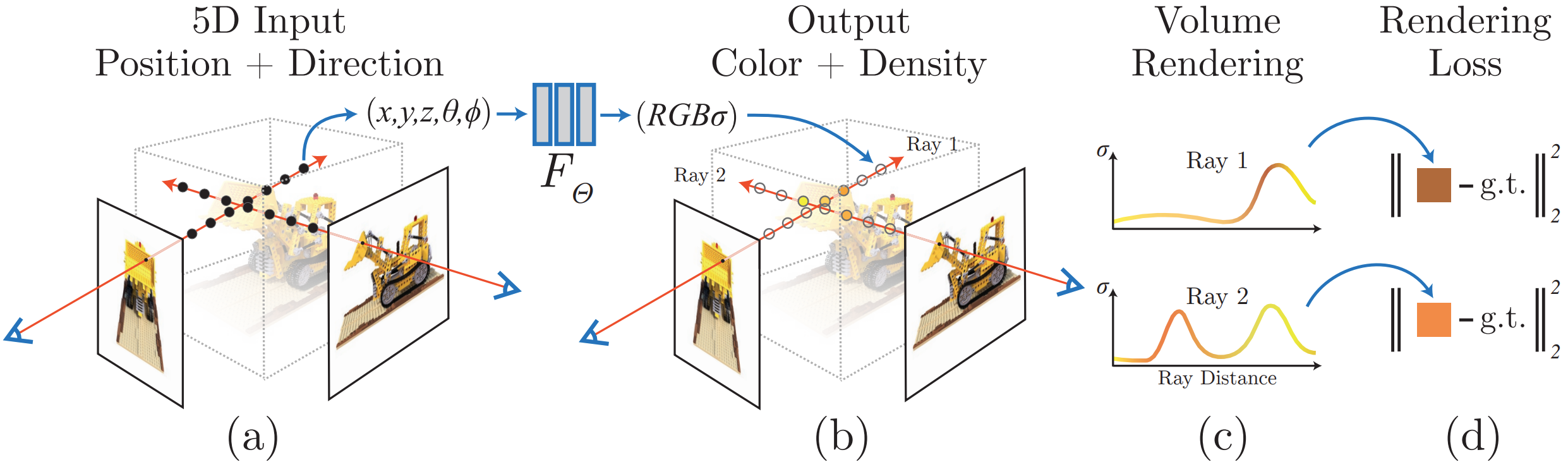
Uses a Neural Network to represent a continuous scene as a $5D$ vector-valued function whose input is a $3D$ location and a $2D$ viewing direction, and whose output is a volume density and emitted color.

$$ f\!\left( \underbrace{x, y, z}_{\text{3D point}},\; \underbrace{\theta, \phi}_{\text{viewing direction}} \right) \;\longrightarrow\; \left( \underbrace{\sigma}_{\text{opacity}},\; \underbrace{\mathbf{c} = (r, g, b)}_{\text{RGB color}} \right) $$

• Sample some pixels from the image to train the model
• Render using NeRF along the ray for that pixel; use an MLP to sample along the ray
• Use a loss (e.g., MSE or PSNR) to compare the rendered output and backpropagate to train

Positional Encoding

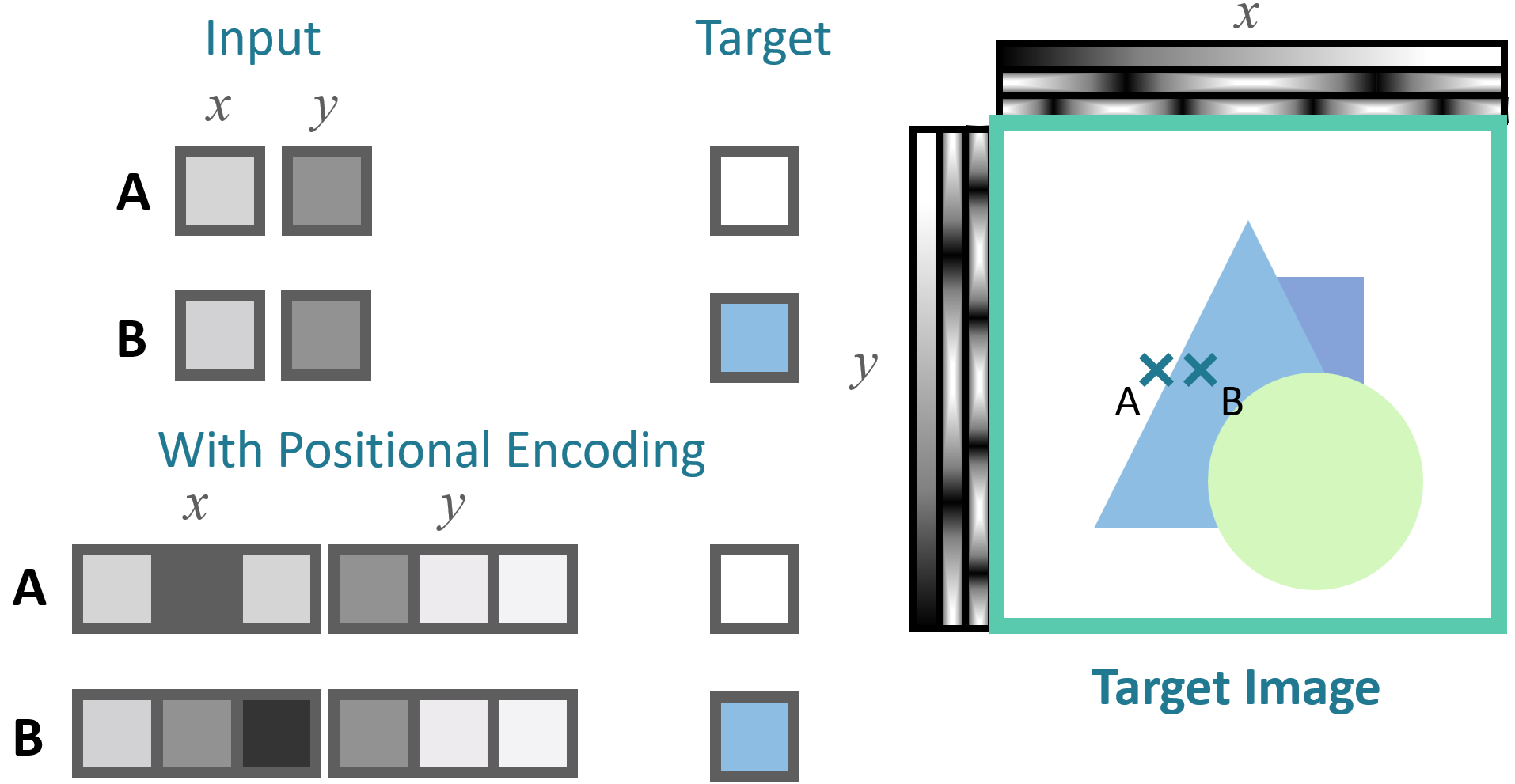
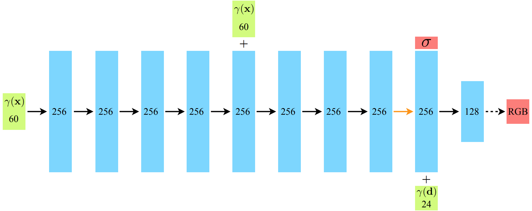
Despite the fact that neural networks are universal function approximators, having the network $F_\Theta$ directly operate on $xyz\theta\phi$ input coordinates results in renderings that perform poorly at representing high-frequency variation in color and geometry because deep networks are biased towards learning lower frequency functions.

Mapping the inputs to a higher dimensional space using high frequency functions before passing them to the network enables better fitting of data that contains high frequency variation.

$$\gamma : \mathbb{R}\rightarrow \mathbb{R}^{2L}$$$$\gamma(p) = (\sin(2^0\pi p), \cos(2^0\pi p), \dots, \sin(2^{L - 1}\pi p), \cos(2^{L - 1}\pi p))$$

This function $\gamma(\cdot)$ is applied separately to each of the three coordinate values in $\mathbf{x}$ which are normalized to lie in $[-1, 1]$ and to the three components of the Cartesian viewing direction unit vector $\mathbf{d}$ (which by construction lie in $[-1, 1]$).

A similar mapping is used in the popular Transformer architecture, where it is referred to as a positional encoding.

---

Hierarchical Sampling

To render using the NeRF we need to sample along the ray for the pixel. A ray is defined as:

$$\mathbf{r}(t) = \underbrace{\mathbf{o}}_{\text{origin}} + t\underbrace{\mathbf{d}}_{\text{direction}}$$

Divide the scene’s $[z_{\text{near}}, z_{\text{far}}]$ into $n$ intervals of equal length. Uniformly sample at random within each interval:

$$ z_i \sim \mathbb{U} \left[ z_n + \frac{(i - 1)(z_{\text{far}} - z_{\text{near}})}{n}, \; z_n + \frac{i (z_{\text{far}} - z_{\text{near}})}{n} \right] $$

Our rendering strategy of densely evaluating the neural radiance field network at $N$ query points along each camera ray is inefficient, free space and occluded regions that do not contribute to the rendered image are still sampled repeatedly.

Instead, simulate two networks: coarse network and fine network.

Sample $N_c$ locations using stratified sampling, and evaluate the coarse network at these locations. Given the output of this network, we then produce a more informed sampling of points along each ray where samples are biased towards the relevant parts of the volume.

To do this, we first rewrite the alpha composited color from the coarse network $\hat{C}_c(\mathbf{r})$ as a weighted sum of all sampled colors $c_i$ along the ray:

$$\hat{C}_c(\mathbf{r}) = \sum_{i=1}^{N_c} w_i c_i, \quad w_i = T_i (1 - \exp(-\sigma_i \delta_i))$$

We can normalize these weights as $\hat{w}_i = \frac{w_i}{\sum_j w_j}$ to produce a piecewise-constant PDF along the ray.

We then sample a second set of $N_f$ locations from this distribution using inverse transform sampling, evaluate the network at the union of first and second set of samples, and compute the final rendered color of ray $\hat{C}_f(\mathbf{r})$ using $N_c + N_f$ samples.

---

Loss Function

During training, the loss is simply the total squared error between the rendered and true pixel colors for both the coarse and fine renderings:

$$\mathcal{L} = \sum_{\mathbf{r}\in \mathcal{R}} \left[ \|\hat{C}_c(\mathbf{r}) - C(\mathbf{r})\|_2^2 + \|\hat{C}_f(\mathbf{r}) - C(\mathbf{r})\|_2^2 \right]$$

where $\mathcal{R}$ is the set of rays in each batch, and $C(\mathbf{r})$, $\hat{C}_c(\mathbf{r})$ and $\hat{C}_f(\mathbf{r})$ are the ground truth, coarse volume predicted and fine volume predicted RGB colors for the ray $\mathbf{r}$ respectively.

Note that even though the final rendering comes from $\hat{C}_f(\mathbf{r})$, we also minimize the loss of $\hat{C}_c(\mathbf{r})$ so that the weight distribution from the coarse network can be used to allocate samples in the fine network.

---

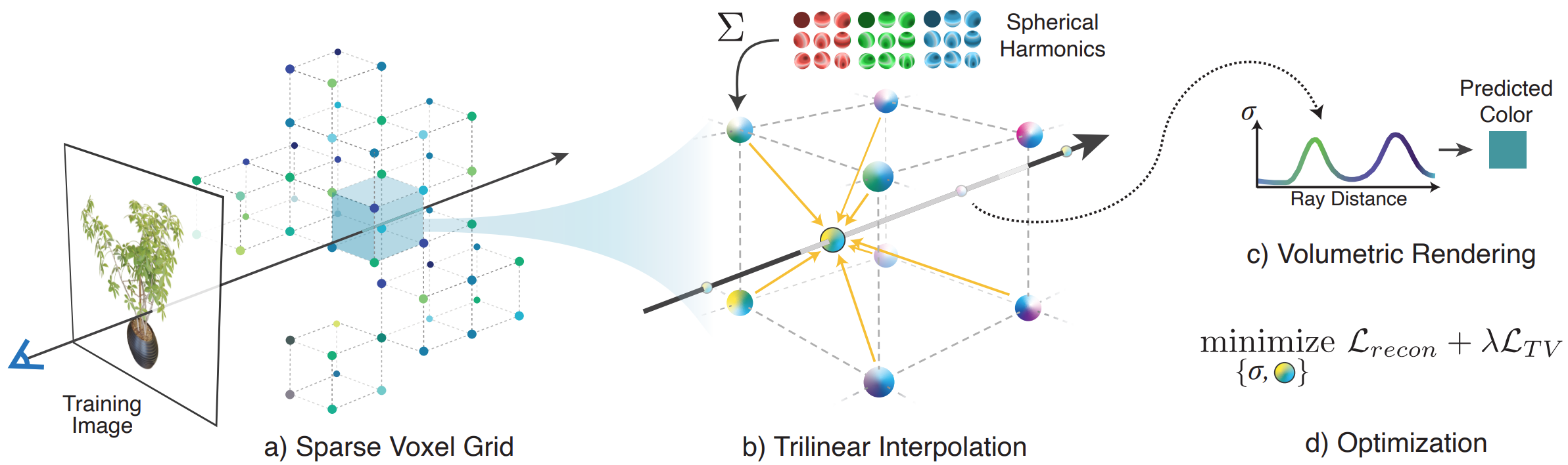
Plenoxels: Radiance Fields without Neural Networks

Overview

In light of the substantial computational requirements of NeRF for both training and rendering, many recent papers have proposed methods to improve efficiency, particularly for rendering.

Method

Plenoxels (plenoptic voxels) represent a scene as a sparse 3D grid with spherical harmonics. This representation can be optimized from calibrated images via gradient methods and regularization without any neural components.

Spherical Harmonics

Uses spherical harmonic coefficients $\mathbf{k}$, rather than RGB values:

$$(\mathbf{k}, \sigma), \quad \mathbf{k} = (k^m_l)_{l: 0 \leq l \leq l_{max}}^{m: -l \leq m \leq l}$$

Each $k_l^m \in \mathbb{R}^{3}$ is a set of 3 coefficients corresponding to RGB components. In this setup, the view-dependent color $\mathbf{c}$ at a point $\mathbf{x}$ may be determined by querying the SH functions $Y_l^m:\mathbb{S}\rightarrow\mathbb{R}$ at desired viewing angle $\mathbf{d}$:

$$c(\mathbf{x}, \mathbf{d}; \mathbf{k}) = \sigma\left( \sum_{l=0}^{l_{max}}\sum_{m=-l}^{l} k_l^m Y_l^m(\mathbf{d}) \right)$$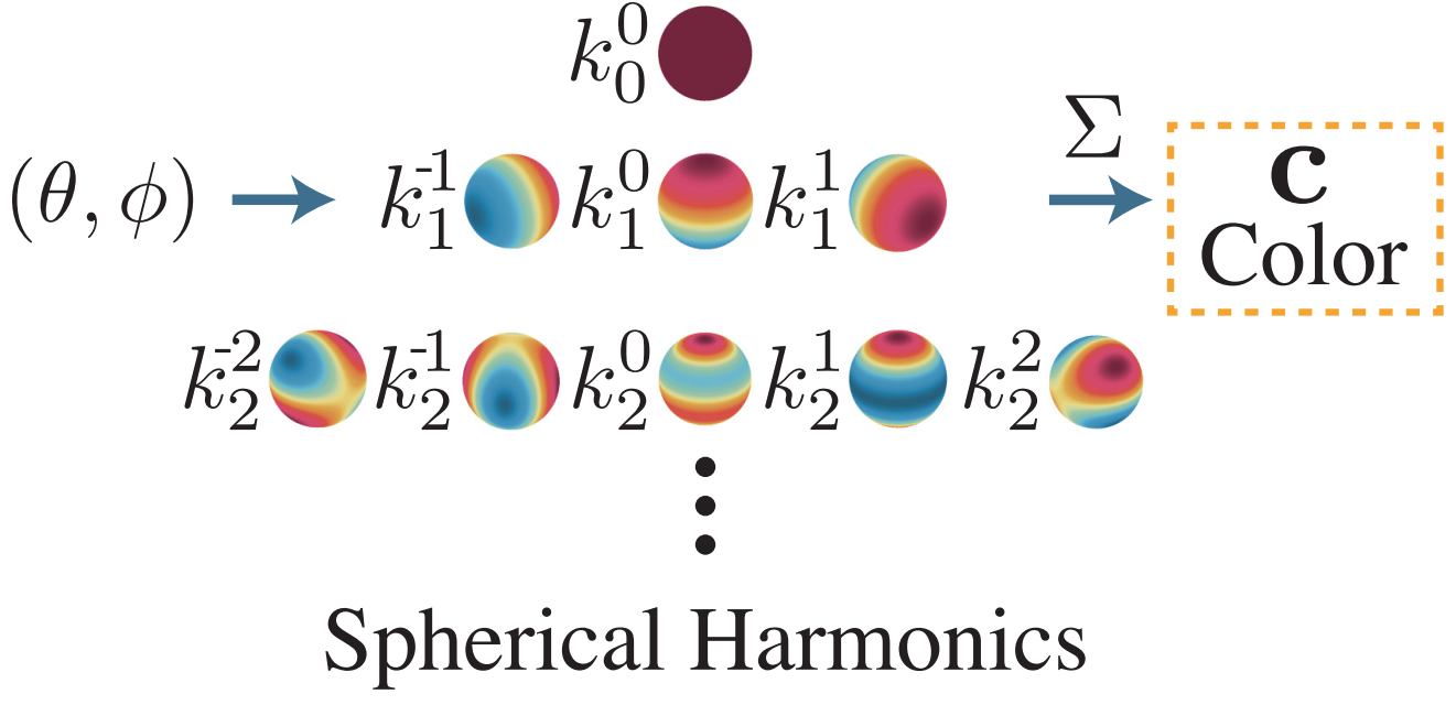

---

Interactive Spherical Harmonics Viewer

Interpolation

So, each vertex of the grid has the SH coefficients and opacity $\sigma$.

The opacity and color at each sample point along ray are computed by trilinear interpolation of opacity and harmonic coefficients stored at nearest 8 voxels.

Coarse to Fine

Achieves high resolution via coarse-to-fine strategy that begins with a dense grid at lower resolution, optimizes, prunes unnecessary voxels, refines the remaining voxels by subdividing each in half in each dimension, and continues optimizing.

Voxel pruning is performed using the method from PlenOctrees Paper here, which applies a threshold to the maximum weight $T_i(1 - \exp(-\sigma_i \delta_i))$ of each voxel over all training ray (or, alternatively, to the density value in each voxel).

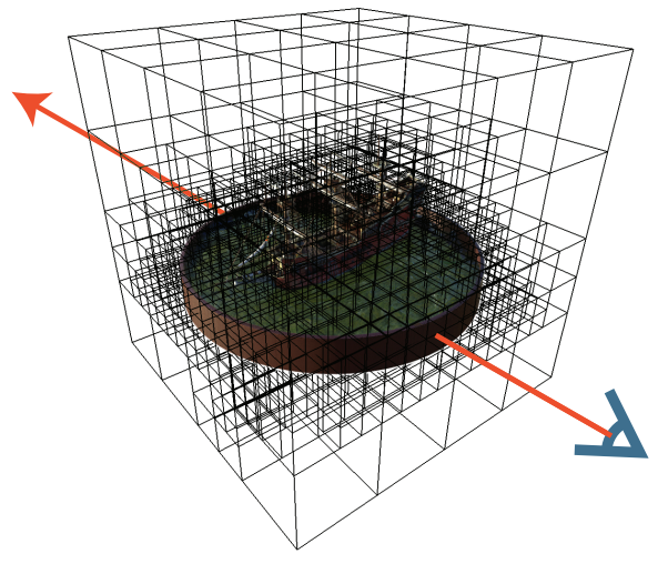
Due to trilinear interpolation, naively pruning can adversely impact the color and density near surfaces since values at these points interpolate with the voxels in the immediate exterior. To solve this, they performed a dilation operation so that voxel is only pruned if both itself and its neighbors are deemed unoccupied.

Interactive PlenOctree

Optimization

Optimize the voxel opacities and spherical harmonic coefficients with respect to the mean squared error (MSE) over rendered pixel colors with total variation (TV) regularization. Specifically, the loss is:

$$\mathcal{L} = \mathcal{L}_{recon} + \lambda_{TV}\mathcal{L}_{TV}$$

where these losses are defined as

$$\mathcal{L}_{\text{recon}}= \frac{1}{|\mathcal{R}|} \sum_{\mathbf{r} \in \mathcal{R}}\left\| C(\mathbf{r}) - \hat{C}(\mathbf{r}) \right\|_2^2 $$$$\mathcal{L}_{\text{TV}} = \frac{1}{|\mathcal{V}|} \sum_{\mathbf{v} \in \mathcal{V}} \sum_{d \in [D]} \sqrt{\Delta_x^2(\mathbf{v}, d)+ \Delta_y^2(\mathbf{v}, d)+ \Delta_z^2(\mathbf{v}, d)}$$

where $ \Delta_x^2(\mathbf{v}, d) $ denotes the squared difference between the $ d^\text{th} $ value in voxel $ \mathbf{v} := (i, j, k) $ and the $ d^\text{th} $ value in voxel $ (i + 1, j, k) $, normalized by the resolution. Analogously, $ \Delta_y^2(\mathbf{v}, d) $ and $ \Delta_z^2(\mathbf{v}, d) $ represent the squared differences along the $ y $- and $ z $-axes, respectively.

Plenoxels achieves significantly faster training than NeRF while maintaining comparable rendering quality since they don’t use neural networks just use differentiable rendering framework.

---

TensoRF

Overview

Unlike NeRF that purely uses MLPs, TensoRF models the radiance field of a scene as a 4D tensor, which represents a 3D voxel grid with per-voxel multi-channel features. The central idea is to factorize the 4D scene tensor into multiple compact low-rank tensor components.

TensoRF presents a novel vector-matrix (VM) decomposition technique that effectively reduces the number of components required for the same expression capacity, leading to faster reconstruction and better rendering than the classic CANDECOMP/PARAFAC (CP) decomposition.

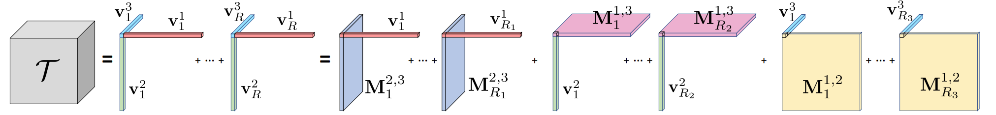
CP Decomposition

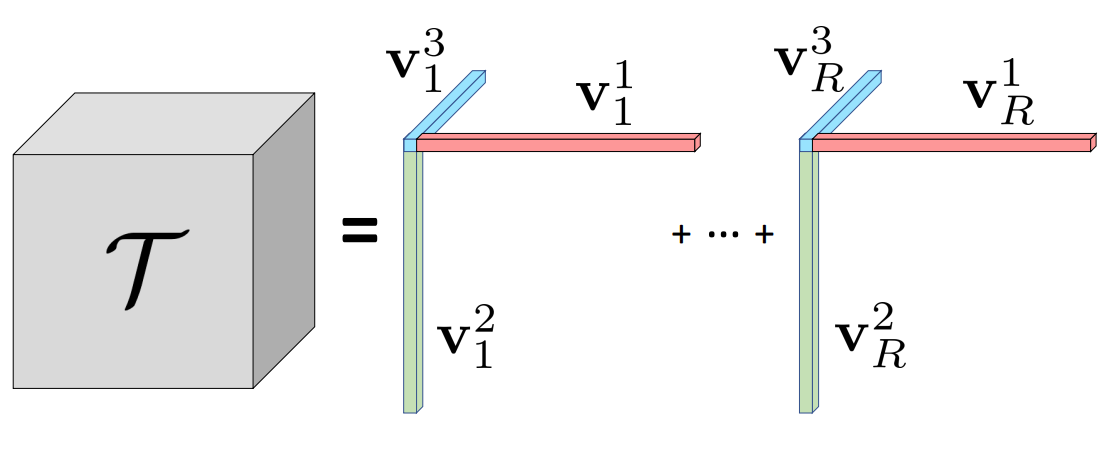
Given a 3D tensor $\mathcal{T} \in \mathbb{R}^{I \times J \times K}$, CP decomposition factorizes it into a sum of outer products of vectors:

$$ \mathcal{T} = \sum_{r=1}^R \mathbf{v}_r^{1} \circ \mathbf{v}_r^{2} \circ \mathbf{v}_r^{3} $$

where $\mathbf{v}_{r}^{1} \circ \mathbf{v}_{r}^{2} \circ \mathbf{v}_r^{3}$ corresponds to a rank-one tensor component, and $\mathbf{v}_r^{1} \in \mathbb{R}^{I}$, $\mathbf{v}_r^{2} \in \mathbb{R}^{J}$, and $\mathbf{v}_r^{3} \in \mathbb{R}^{K}$ are factorized vectors of the three modes for the $r^\text{th}$ component. Superscripts denote the modes of each factor; $\circ$ represents the outer product. Hence, each tensor element $\mathcal{T}_{ijk}$ is a sum of scalar products:

$$ \mathcal{T}_{ijk} = \sum_{r=1}^R \mathbf{v}_{r,i}^{1} \mathbf{v}_{r,j}^{2} \mathbf{v}_{r,k}^{3} $$

where $i, j, k$ denote the indices of the three modes.

CP decomposition factorizes a tensor into multiple vectors, expressing multiple compact rank-one components. However, because of too high compactness, CP decomposition can require many components to model complex scenes, leading to high computational costs in radiance field reconstruction.

Vector-Matrix (VM) Decomposition

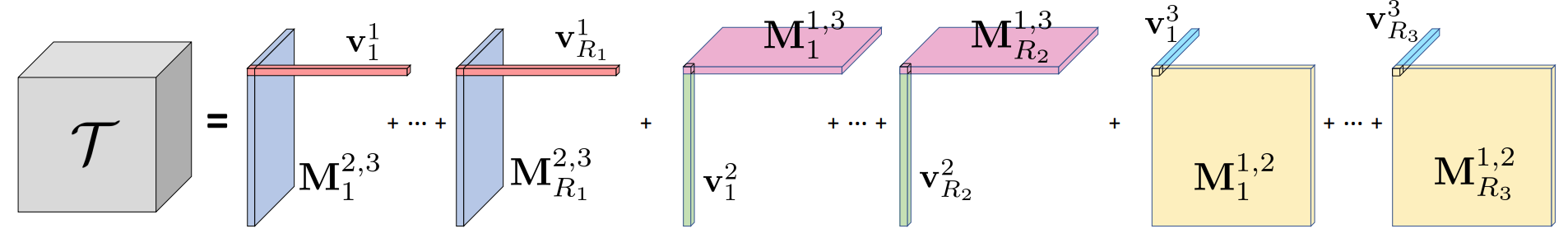
Unlike CP decomposition that utilizes pure vector factors, VM decomposition factorizes a tensor into multiple vectors and matrices. This is expressed by:

$$ \mathcal{T} = \sum_{r=1}^{R_1} \mathbf{v}_r^{1} \circ \mathbf{M}_r^{2,3} + \sum_{r=1}^{R_2} \mathbf{v}_r^{2} \circ \mathbf{M}_r^{1,3} + \sum_{r=1}^{R_3} \mathbf{v}_r^{3} \circ \mathbf{M}_r^{1,2} $$

where $\mathbf{M}_r^{2,3} \in \mathbb{R}^{J \times K}$, $\mathbf{M}_r^{1,3} \in \mathbb{R}^{I \times K}$, and $\mathbf{M}_r^{1,2} \in \mathbb{R}^{I \times J}$ are matrix factors for two (denoted by superscripts) of the three modes.

For each component, we relax its two mode ranks to be arbitrarily large, while restricting the third mode to be rank-one; e.g., for component tensor $\mathbf{v}_r^{1} \circ \mathbf{M}_r^{2,3}$, its mode-1 rank is 1, and its mode-2 and mode-3 ranks can be arbitrary, depending on the rank of the matrix $\mathbf{M}_r^{2,3}$.

Comparison

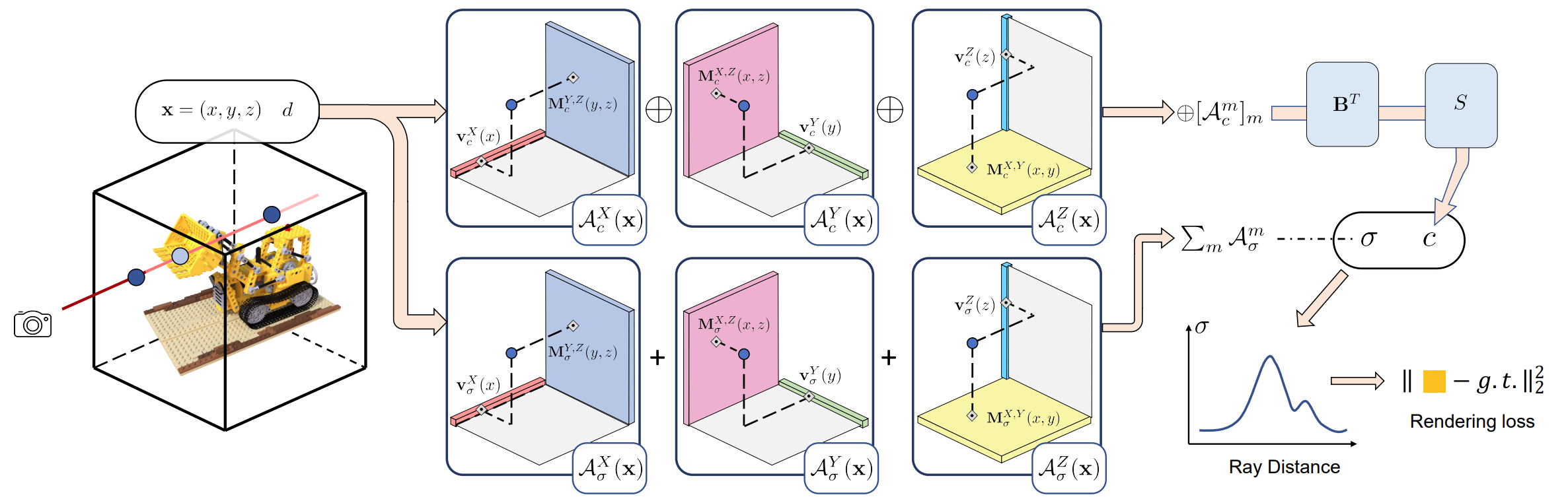
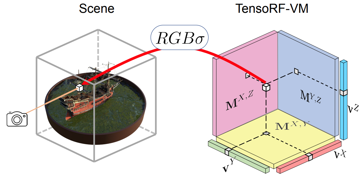
Tensor for Scene Modeling

In this work, we focus on the task of modeling and reconstructing radiance fields. We can view the image below. In this case, the three tensor modes correspond to the XYZ axes, and we thus directly denote the modes with XYZ to make it intuitive. Meanwhile, in the context of 3D scene representation, we consider $R_1 = R_2 = R_3 = R$ for most scenes, reflecting the fact that a scene can distribute and appear equally complex along its three axes. Therefore, the previous equation can be re-written as:

$$ \mathcal{T} = \sum_{r=1}^{R} \mathbf{v}_r^{X} \circ \mathbf{M}_r^{Y,Z} + \mathbf{v}_r^{Y} \circ \mathbf{M}_r^{X,Z} + \mathbf{v}_r^{Z} \circ \mathbf{M}_r^{X,Y} $$

In addition, to simplify notation and the following discussion in later sections, we also denote the three types of component tensors as $A_r^{X} = \mathbf{v}_r^{X} \circ \mathbf{M}_r^{Y,Z}$, $A_r^{Y} = \mathbf{v}_r^{Y} \circ \mathbf{M}_r^{X,Z}$, and $A_r^{Z} = \mathbf{v}_r^{Z} \circ \mathbf{M}_r^{X,Y}$; here the superscripts XYZ of $A$ indicate different types of components.

With this, a tensor element $\mathcal{T}_{ijk}$ is expressed as:

$$ \mathcal{T}_{ijk} = \sum_{r=1}^{R} \sum_{m} \mathcal{A}_{r,ijk}^{m} $$

where $m \in \{X, Y, Z\}$, $A_{r,ijk}^{X} = v_{r,i}^{X} M_{r,jk}^{Y,Z}$, $A_{r,ijk}^{Y} = v_{r,j}^{Y} M_{r,ik}^{X,Z}$, and $A_{r,ijk}^{Z} = v_{r,k}^{Z} M_{r,ij}^{X,Y}$.

Feature Grids and Radiance Field

We leverage a regular 3D grid G with per-voxel multi-channel features to model such a function. We split it (by feature channels) into a geometry grid $\mathcal{G}_{\sigma}$ and an appearance grid $\mathcal{G}_{c}$, separately modelling the volume density $\sigma$ and view-dependent color $c$:

$$ \sigma, c = \mathcal{G}_{\sigma}(\mathbf{x}), \; \underbrace{\mathcal{S}(\mathcal{G}_{c}(\mathbf{x}), d)}_{\text{it can be MLP/SH}} $$

where $\mathcal{G}_{\sigma}(\mathbf{x})$, $\mathcal{G}_{c}(\mathbf{x})$ represent the trilinearly interpolated features from the two grids at location $\mathbf{x}$. We model $\mathcal{G}_{\sigma}$ and $\mathcal{G}_{c}$ as factorized tensors.

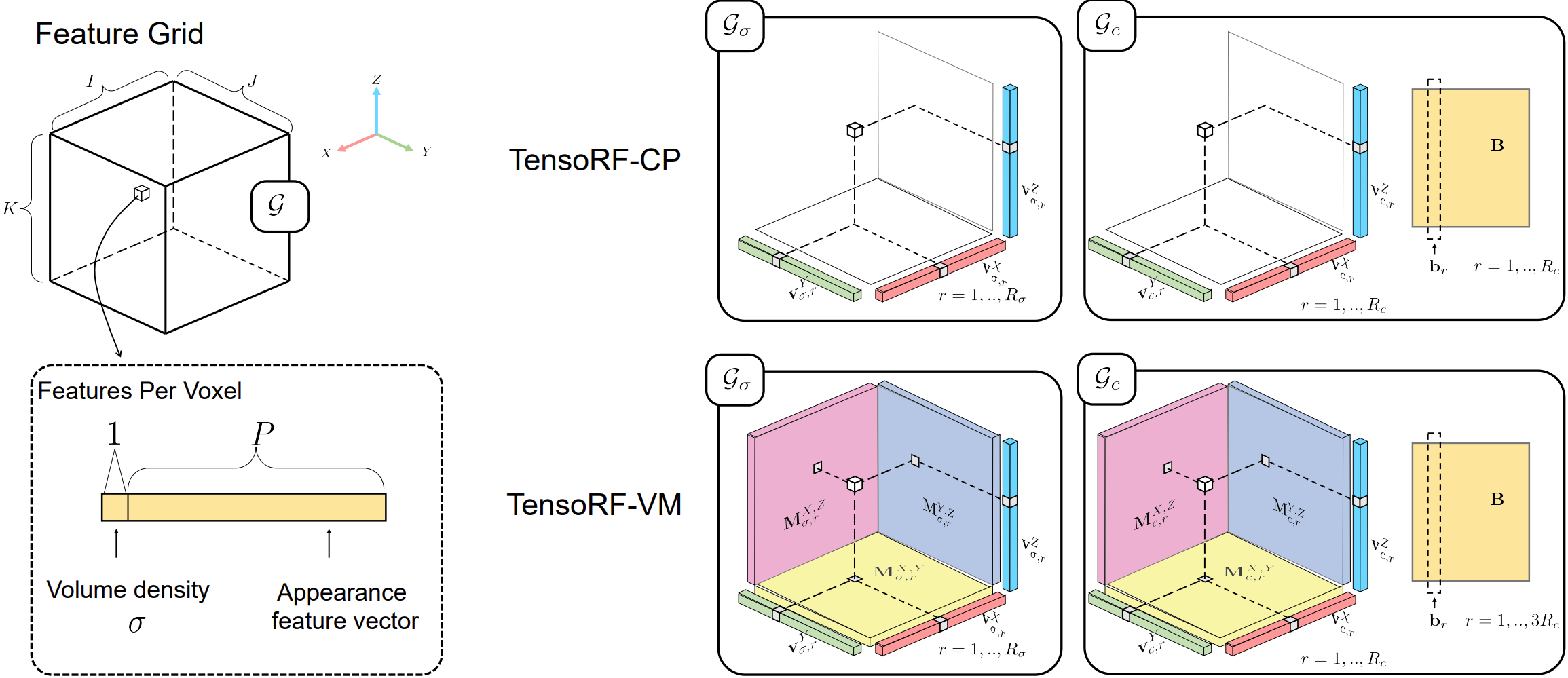
Factorizing Radiance Fields

While $\mathcal{G}_{\sigma} \in \mathbb{R}^{I \times J \times K}$ is a 3D tensor, $\mathcal{G}_{c} \in \mathbb{R}^{I \times J \times K \times P}$ is a 4D tensor. Here $I, J, K$ correspond to the resolutions of the feature grid along the X, Y, Z axes, and $P$ is the number of appearance feature channels.

We factorize these radiance field tensors to compact components. In particular, with the VM decomposition, the 3D geometry tensor $\mathcal{G}_{\sigma}$ is factorized as:

$$ \mathcal{G}_{\sigma} = \sum_{r=1}^{R_{\sigma}} \mathbf{v}_{\sigma,r}^{X} \circ \mathbf{M}_{\sigma,r}^{Y,Z} + \mathbf{v}_{\sigma,r}^{Y} \circ \mathbf{M}_{\sigma,r}^{X,Z} + \mathbf{v}_{\sigma,r}^{Z} \circ \mathbf{M}_{\sigma,r}^{X,Y} = \sum_{r=1}^{R_{\sigma}} \sum_{m \in \{X,Y,Z\}} \mathcal{A}_{\sigma,r}^{m} $$

The appearance tensor $\mathcal{G}_{c}$ has an additional mode corresponding to the feature channel dimension:

$$ \mathcal{G}_{c} = \sum_{r=1}^{R_{c}} \mathbf{v}_{c,r}^{X} \circ \mathbf{M}_{c,r}^{Y,Z} \circ \mathbf{b}_{3r-2} + \mathbf{v}_{c,r}^{Y} \circ \mathbf{M}_{c,r}^{X,Z} \circ \mathbf{b}_{3r-1} + \mathbf{v}_{c,r}^{Z} \circ \mathbf{M}_{c,r}^{X,Y} \circ \mathbf{b}_{3r} $$$$ = \sum_{r=1}^{R_{c}} \mathcal{A}_{c,r}^{X} \circ \mathbf{b}_{3r-2} + \mathcal{A}_{c,r}^{Y} \circ \mathbf{b}_{3r-1} + \mathcal{A}_{c,r}^{Z} \circ \mathbf{b}_{3r} $$

Note that we have $3R_{c}$ vectors $\mathbf{b}_{r}$ to match the total number of components.

Overall, we factorize the entire tensorial radiance field into $3R_{\sigma} + 3R_{c}$ matrices ($\mathbf{M}_{\sigma,r}^{Y,Z}, \ldots, \mathbf{M}_{c,r}^{Y,Z}, \ldots$) and $3R_{\sigma} + 6R_{c}$ vectors ($\mathbf{v}_{\sigma,r}^{X}, \ldots, \mathbf{v}_{c,r}^{X}, \ldots, \mathbf{b}_{r}$).

In general, we adopt $R_{\sigma} \ll I, J, K$ and $R_{c} \ll I, J, K$, leading to a highly compact representation that can encode a high-resolution dense grid.

In essence, the XYZ-mode vector and matrix factors $\mathbf{v}_{\sigma,r}^{X}, \mathbf{M}_{\sigma,r}^{Y,Z}, \mathbf{v}_{c,r}^{X}, \mathbf{M}_{c,r}^{Y,Z}, \ldots$ describe the spatial distributions of the scene geometry and appearance along their corresponding axes. On the other hand, the appearance feature-mode vectors $\mathbf{b}_{r}$ express the global appearance correlations.

By stacking all $\mathbf{b}_{r}$ as columns together, we have a $P \times 3R_{c}$ matrix $\mathbf{B}$; this matrix $\mathbf{B}$ can also be seen as a global appearance dictionary that abstracts the appearance commonalities across the entire scene.

Interpolation

Naively achieving trilinear interpolation is costly, as it requires evaluation of 8 tensor values and interpolating them, increasing computation by a factor of 8 compared to computing a single tensor element. However, we find that trilinearly interpolating a component tensor is naturally equivalent to interpolating its vector/matrix factors linearly/bilinearly for the corresponding modes, thanks to the beauty of linearity of the trilinear interpolation and the outer product.

---

Interactive Overview of TensoRF

Rendering Process

For a 3D point $\mathbf{x}$ and viewing direction $\mathbf{d}$:

1. Interpolate geometry features:

   $$\mathbf{f}_{\sigma} = \text{interp}(\mathcal{G}_{\sigma}, \mathbf{x})$$

2. Compute density:

   $$\sigma(\mathbf{x}) = \text{ReLU}(\mathbf{f}_{\sigma})$$

3. Interpolate appearance features:

   $$\mathbf{f}_{c} = \text{interp}(\mathcal{G}_{c}, \mathbf{x})$$

4. Predict color with small MLP or SH:

   $$\mathbf{c}(\mathbf{x}, \mathbf{d}) = \text{MLP/SH}([\mathbf{f}_{c}, \mathbf{d}])$$

Training Objective

The optimization minimizes a composite loss:

$$ \mathcal{L} = \mathcal{L}_{\text{recon}} + \lambda_{\text{TV}} \mathcal{L}_{\text{TV}} $$

where:

• Reconstruction loss: $\mathcal{L}_{\text{recon}} = \|\mathbf{C} - \hat{\mathbf{C}}\|_2^2$ (MSE between rendered and ground truth colors)
• Total Variation (TV) regularization: $\mathcal{L}_{\text{TV}}$ encourages spatial smoothness in the vector and matrix factors:

$$ \mathcal{L}_{\text{TV}} = \sum_{r} \left( \|\nabla \mathbf{v}_r\|_1 + \|\nabla \mathbf{M}_r\|_1 \right) $$

TV regularization prevents overfitting and removes floaters/artifacts by enforcing piecewise-smooth geometry and appearance.

---

Instant NGP

Overview

Given a fully connected neural network $m(y; \Phi)$, we are interested in an encoding of its inputs $y = \text{enc}(x; \theta)$ that improves the approximation quality and training speed across a wide range of applications without incurring a notable performance overhead.

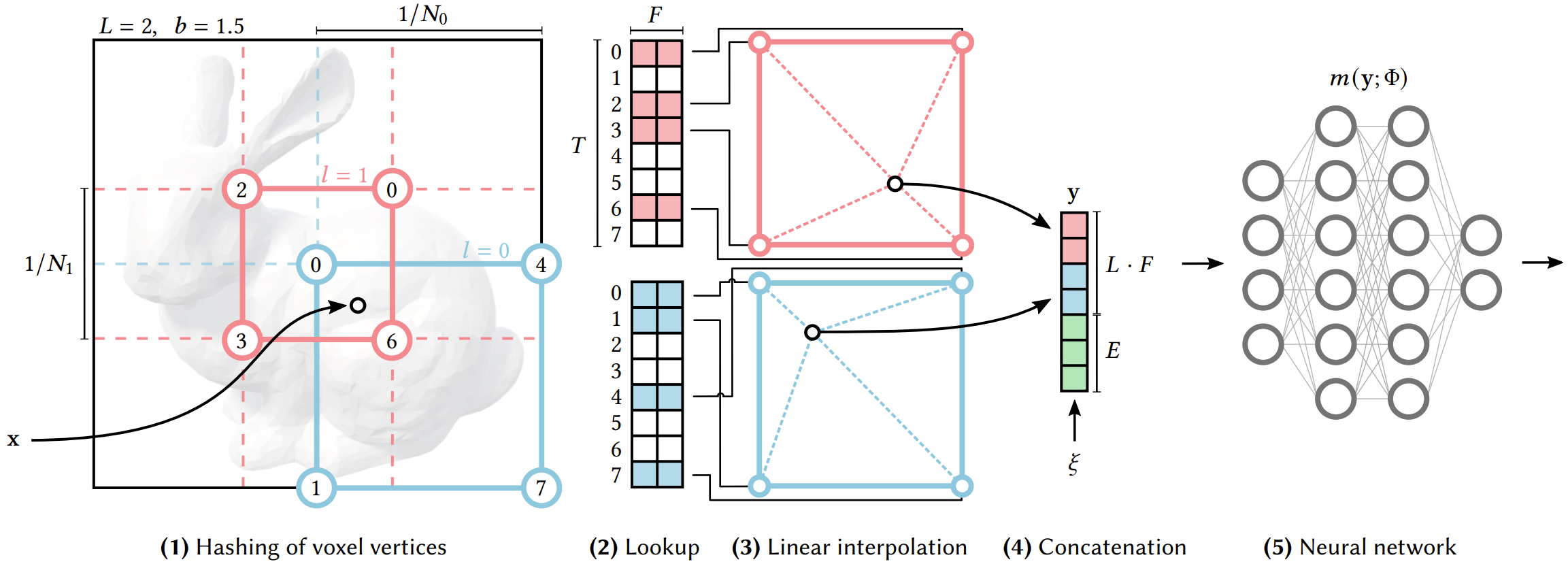
Multiresolution Hash Encoding

Our neural network not only has trainable weight parameters $\Phi$, but also trainable encoding parameters $\theta$. These are arranged into $L$ levels, each containing up to $T$ feature vectors with dimensionality $F$.

Each level (two of which are shown as red and blue in the figure) is independent and conceptually stores feature vectors at the vertices of a grid, the resolution of which is chosen to be a geometric progression between the coarsest and finest resolutions $[N_{\min}, N_{\max}]$:

$$ N_l := \left\lfloor N_{\min} \cdot b^{\,l} \right\rfloor, $$$$ b := \exp\!\left( \frac{\ln N_{\max} - \ln N_{\min}}{L - 1} \right). $$

$N_{\max}$ is chosen to match the finest detail in the training data. Due to the large number of levels $L$, the growth factor is usually small.

Interactive Demo for Multi Resolution Hash Encoding

Growth Factor Derivation

To create a geometric progression of resolutions from $N_{\min}$ to $N_{\max}$ over $L$ levels:

$$N_l = N_{\min} \cdot b^l \quad \text{for } l = 0, 1, \ldots, L-1$$

At the finest level ($l = L-1$), we want $N_{L-1} = N_{\max}$:

$$N_{\min} \cdot b^{L-1} = N_{\max}$$

Solving for $b$:

$$b^{L-1} = \frac{N_{\max}}{N_{\min}}$$

Take natural log of both sides:

$$(L-1) \ln(b) = \ln(N_{\max}) - \ln(N_{\min})$$

Therefore:

$$b = \exp\left(\frac{\ln N_{\max} - \ln N_{\min}}{L - 1}\right)$$

Intuition: We have $L$ levels, requiring $(L-1)$ multiplicative steps. The formula ensures each level’s resolution is exactly $b$ times the previous level, creating a smooth exponential growth from coarse to fine detail.

We map each corner to an entry in the level’s respective feature vector array, which has a fixed size of at most $T$. For coarse levels where a dense grid requires fewer than $T$ parameters, i.e. $(N_l + 1)^d \leq T$, this mapping is $1\!:\!1$.

At finer levels, we use a hash function $h : \mathbb{Z}^d \rightarrow \mathbb{Z}_T$ to index into the array, effectively treating it as a hash table, although there is no explicit collision handling. We rely instead on the gradient-based optimization to store appropriate sparse detail in the array, and the subsequent neural network $m(y; \Phi)$ for collision resolution.

The number of trainable encoding parameters $\theta$ is therefore $\mathcal{O}(T)$ and bounded by $T \cdot L \cdot F$.

The spatial hash function has the form:

$$ h(\mathbf{x}) = \left( \sum_{i=1}^{d} x_i \, \pi_i \right) \bmod T, $$

where $\pi_i$ are unique large prime numbers (e.g., $\pi_1 = 1$, $\pi_2 = 2654435761$, $\pi_3 = 805459861$).

Feature Lookup and Interpolation

For a query point $\mathbf{x}$, the encoding process at each resolution level $l$ involves:

1. Identify surrounding voxel: Find the 8 corner vertices of the voxel containing $\mathbf{x}$ at resolution $N_l$
2. Hash each corner: Apply $h(\mathbf{x}_i)$ to each of the 8 corners to get indices into the hash table
3. Retrieve features: Look up the $F$-dimensional feature vectors $\mathbf{f}_i \in \mathbb{R}^F$ from the hash table
4. Trilinear interpolation: Interpolate features based on $\mathbf{x}$’s position within the voxel:

$$ \mathbf{y}_l = \text{trilinear}\left(\{\mathbf{f}_i\}_{i=1}^{8}, \mathbf{x}\right) \in \mathbb{R}^F $$

5. Concatenate across all levels: The final encoded representation is:

$$ y = \text{enc}(\mathbf{x}; \theta) = [\mathbf{y}_1, \mathbf{y}_2, \ldots, \mathbf{y}_L] \in \mathbb{R}^{L \cdot F} $$

This encoded feature vector $y$ is then fed to the MLP $m(y; \Phi)$ for final prediction.

Network Architecture

After hash encoding, a compact MLP processes the concatenated features. For NeRF applications:

• Input: Encoded position features $y \in \mathbb{R}^{L \cdot F}$ concatenated with viewing direction $\mathbf{d}$
• Architecture: 2 hidden layers with 64 neurons each (vs. original NeRF’s 8 layers × 256 neurons)
• Activation: ReLU
• Output: RGB color $\mathbf{c} \in \mathbb{R}^3$ and volume density $\sigma \in \mathbb{R}$

The forward pass is:

$$ \mathbf{c}, \sigma = m\left([\text{enc}(\mathbf{x}; \theta), \mathbf{d}]; \Phi\right) $$

The dramatically smaller network (2 layers vs 8) is enabled by the expressive hash encoding, which offloads spatial feature learning from the MLP to the trainable hash table.

Collision Handling

When multiple voxel corners hash to the same index in the hash table (a collision), no explicit resolution mechanism is used. Instead:

• Multi-resolution disambiguation: The same 3D location maps to different indices at different resolution levels, providing redundancy
• Neural disambiguation: The MLP $m(y; \Phi)$ learns to interpret ambiguous/collided features correctly during training
• Gradient-based prioritization: Backpropagation naturally stores important features where gradients are high, while collisions in low-gradient regions have minimal impact
• Sparse detail: The optimization focuses hash table capacity on regions with fine detail, letting collisions occur in smooth/empty areas

This implicit collision handling is what allows a fixed-size hash table ($T \approx 2^{19}$ entries) to represent arbitrarily fine detail without explicit collision resolution overhead.

Hyperparameter Configuration

Typical values for NeRF applications:

• Hash table size: $T = 2^{19}$ (~524K entries)
• Feature dimension: $F = 2$ per level
• Number of levels: $L = 16$
• Resolution range: $N_{\min} = 16$, $N_{\max} = 2048$
• Total encoding parameters: $T \cdot L \cdot F \approx 16.8$ million

Total trainable parameters (encoding + MLP) is still much smaller than original NeRF while achieving 20-60× faster training.

---

3DGS

Overview

The input to the method is a set of images of a static scene, together with the corresponding cameras calibrated by Structure-from-Motion (SfM), which produces a sparse point cloud as a side-effect.

Gaussian Parametrization

From these sparse points, a set of 3D Gaussians is created, where each Gaussian is parametrized by:

$$\mu \in \mathbb{R}^{3}: \text{center position (mean)}$$$$r \in \mathbb{R}^{4}: \text{rotation (using quaternion representation)}$$$$s \in \mathbb{R}^{3}: \text{scale factors}$$

The covariance matrix $\Sigma \in \mathbb{R}^{3\times 3}$ is decomposed as:

$$\Sigma = RSS^TR^T$$

where:

• $S \in \mathbb{R}^{3 \times 3}$ is a diagonal scaling matrix: $S = \text{diag}(s_x, s_y, s_z)$
• $R \in SO(3)$ is a rotation matrix constructed from quaternion $r$: $R = \text{q2R}(r)$

This parametrization ensures the covariance $\Sigma$ is positive semi-definite (PSD), which is required for valid Gaussians.

Rendering using Gaussians

3DGS uses spherical harmonics (SH) to encode view-dependent appearance and uses $\alpha$-blending. Point-based $\alpha$-blending and NeRF-style volumetric rendering share essentially the same image formation model. The color $C$ along a ray is given by:

$$ C = \sum_{i=1}^{N} T_i (1 - \exp(-\sigma_i \delta_i)) c_i \quad \text{with} \quad T_i = \exp\left(-\sum_{j=1}^{i-1} \sigma_j \delta_j\right) $$

where samples of density $\sigma$, transmittance $T$, and color $\mathbf{c}$ are taken along the ray with intervals $\delta_i$. This can be rewritten as:

$$ C = \sum_{i=1}^{N} T_i \alpha_i \mathbf{c}_i $$

with

$$ \alpha_i = (1 - \exp(-\sigma_i \delta_i)) \quad \text{and} \quad T_i = \prod_{j=1}^{i-1} (1 - \alpha_j) $$

For each pixel, the color and opacity of $N$ overlapping Gaussians are combined as:

$$ C = \sum_{i=1}^{N}c_i\alpha_i\prod_{j=1}^{i - 1}(1 - \alpha_j) $$

The $\alpha_i$ value for each Gaussian is computed as:

$$\alpha_i = o_i \cdot e^{-\frac{1}{2}(\mathbf{x} - \mu_i)^T \Sigma_i^{-1} (\mathbf{x} - \mu_i)}$$

where $o_i$ is the learned opacity parameter, ensuring $\alpha_i$ decreases as we move away from the Gaussian center $\mu_i$.

Projection to Screen Space

To render 3D Gaussians, they must be projected to 2D screen space. Given camera extrinsic matrix $T$ and intrinsic matrix $K$:

$$\hat{\mu} = KT[\mu, 1]^T$$

$$\hat{\Sigma} = J W \Sigma W^T J^T$$

where:

• $\hat{\mu}:$ 2D position on screen
• $\hat{\Sigma}:$ 2D covariance in screen space
• $J:$ Jacobian of the projection
• $W:$ the $3\times3$ rotation component of the world-to-camera transformation

Proof

We start with a Gaussian defined in world space:

$$ X_w \sim \mathcal N(\mu_w, \Sigma). $$

This means:

• $\mathbb E[X_w] = \mu_w$
• $\mathrm{Cov}(X_w) = \Sigma \in \mathbb R^{3\times 3}$

Transform Gaussian into camera space

The world→camera transform is an affine map:

$$ X_c = W X_w + t. $$

Since $t$ is constant, it does not affect covariance.
Using the affine Gaussian rule:

If $X \sim \mathcal N(\mu, \Sigma)$ and $Y = A X + b$, then
$\mathrm{Cov}(Y) = A \Sigma A^\top$. we obtain:

$$ \mu_c = W \mu_w + t, \qquad \Sigma_c = W \Sigma W^\top. $$

Thus:

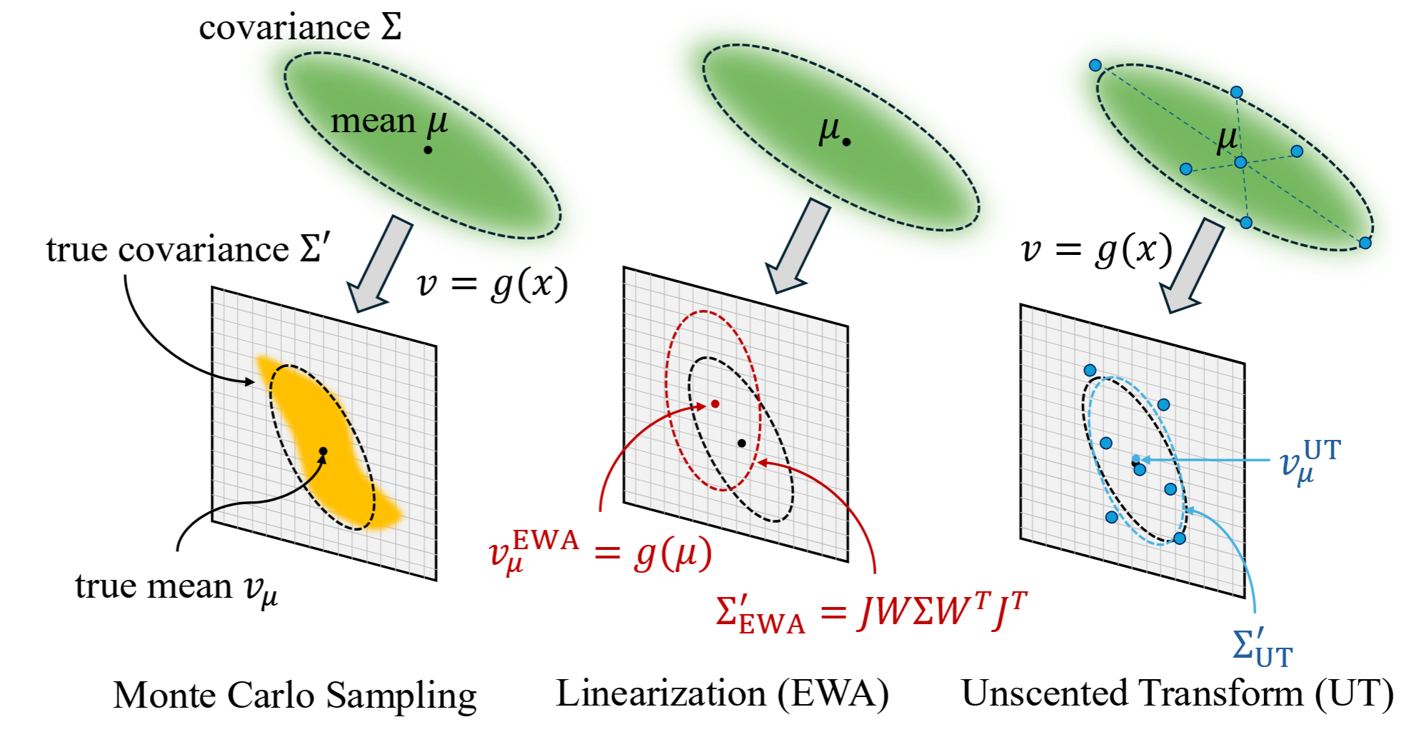
$$ X_c \sim \mathcal N(\mu_c,\, W\Sigma W^\top). $$

Linearize the camera projection

Let the projection be:

$$ f: \mathbb R^3 \to \mathbb R^2, \quad Y = f(X_c). $$

Because $f$ is nonlinear (from division by depth), the distribution of $f(X_c)$ is not Gaussian.
We use the first-order Taylor expansion of $f$ at the mean $\mu_c$:

$$ f(X_c) \approx f(\mu_c) + J(\mu_c)(X_c - \mu_c), $$

where the Jacobian is:

$$ J = \left. \frac{\partial f}{\partial X_c} \right|_{X_c = \mu_c}. $$

Ignoring the constant term $f(\mu_c)$ for covariance gives the linearized random variable:

$$ Y_{\text{lin}} = J(X_c - \mu_c). $$

Propagate the covariance

Using $\mathrm{Cov}(A Z) = A\,\mathrm{Cov}(Z)\,A^\top$:

$$ \Sigma' = \mathrm{Cov}(Y_{\text{lin}}) = J\,\mathrm{Cov}(X_c - \mu_c)\,J^\top. $$

Since subtracting the mean does not affect covariance:

$$ \mathrm{Cov}(X_c - \mu_c) = \mathrm{Cov}(X_c) = \Sigma_c, $$

we get:

$$ \Sigma' = J \Sigma_c J^\top. $$

Substituting $\Sigma_c = W\Sigma W^\top$:

$$ \boxed{\Sigma' = J ( W \Sigma W^\top ) J^\top }. $$

The full chain of transformations is:

$$ X_w \;\longrightarrow\; X_c = W X_w + t \;\longrightarrow\; Y \approx f(\mu_c) + J(X_c - \mu_c). $$

and the covariance flow is:

$$ \Sigma \;\longrightarrow\; W \Sigma W^\top \;\longrightarrow\; J(W \Sigma W^\top) J^\top. $$

Thus, under first-order projection, the 3D Gaussian ellipsoid becomes a 2D Gaussian ellipse with covariance $\Sigma'$.

This EWA (Elliptical Weighted Average) splatting ensures Gaussians remain elliptical after projection.

Adaptive Density Control

Starting from the initial sparse SfM point cloud, the method adaptively controls the number of Gaussians and their density through densification and pruning operations.

Two main scenarios require density adjustment:

• Under-reconstruction: Regions with missing geometric features
• Over-reconstruction: Regions where Gaussians cover excessively large areas

Clone (Under-Reconstruction)

For under-reconstructed regions, Gaussians with high positional gradients are cloned: a copy is created and moved in the direction of the positional gradient.

Split (Over-Reconstruction)

For over-reconstructed regions with large Gaussians:

• Replace the original Gaussian with two smaller ones
• Divide each scale component by 1.6 (as specified in the paper)
• Initialize positions by sampling from the PDF of the original Gaussian

Pruning

Gaussians are removed to maintain efficiency:

• Remove Gaussians with opacity $o < \epsilon$ (typically $\epsilon = 0.005$)
• Reset opacity to near-zero every $K$ iterations (typically 3000 iterations) to force re-optimization
• Remove Gaussians that are excessively large in world space

---

Algorithm: Optimization and Densification

$w, h$: width and height of the training images

---

$M \leftarrow$ SfM Points	▷ Positions
$S, C, A \leftarrow$ InitAttributes()	▷ Covariances, Colors, Opacities
$i \leftarrow 0$	▷ Iteration Count
while not converged do
$V, \hat{I} \leftarrow$ SampleTrainingView()	▷ Camera $V$ and Image
$I \leftarrow$ Rasterize$(M, S, C, A, V)$
$L \leftarrow$ Loss$(I, \hat{I})$	▷ Loss
$M, S, C, A \leftarrow$ Adam$(\nabla L)$	▷ Backprop & Step
if IsRefinementIteration$(i)$ then
for all Gaussians $(\mu, \Sigma, c, \alpha)$ in $(M, S, C, A)$ do
if $\alpha < \epsilon$ or IsTooLarge$(\mu, \Sigma)$ then	▷ Pruning
RemoveGaussian()
end if
if $\nabla_p L > \tau_p$ then	▷ Densification
if $\|S\| > \tau_S$ then	▷ Over-reconstruction
SplitGaussian$(\mu, \Sigma, c, \alpha)$
else	▷ Under-reconstruction
CloneGaussian$(\mu, \Sigma, c, \alpha)$
end if
end if
end for
end if
$i \leftarrow i + 1$
end while

---

Training Loss

The optimization uses a combination of L1 and SSIM losses:

$$\mathcal{L} = (1 - \lambda)\mathcal{L}_1 + \lambda \mathcal{L}_{\text{D-SSIM}}$$

where $\lambda = 0.2$. This balances:

• L1 loss: Pixel-wise color difference
• D-SSIM: Structural similarity (captures perceptual quality)

Interactive Gaussian Viewer

---

Sparse Input

Depth-supervised NeRF

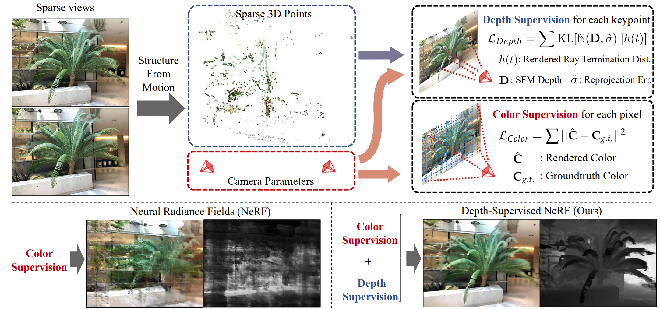
A commonly observed failure mode of Neural Radiance Field (NeRF) is fitting incorrect geometries when given an insufficient number of input views. One potential reason is that standard volumetric rendering does not enforce the constraint that most of a scene’s geometry consist of empty space and opaque surfaces.

Overview

Key idea Leverage the fact that current NeRF pipelines require images with known camera poses that are typically estimated by running structure-from-motion (SFM), which also produces sparse 3D points that can be used as “free” depth super- vision during training:

Volumetric Rendering Revisited

To render a 2D image given a pose $P$, we cast rays $r(t)$ originating from the center of projection $o$ in directions $d$ derived from its intrinsics. We then integrate the implicit radiance field along each ray to compute the incoming radiance contributed by any object intersected along $d$:

$$ C = \int_{0}^{\infty} T(t)\,\sigma(t)\,c(t)\,dt. $$

Here, $t$ parameterizes the aforementioned ray as $r(t) = o + t d$, and $T(t) = \exp\!\left(-\int_0^{t} \sigma(s)\, ds\right)$ checks for occlusions by integrating the differential density from $0$ to $t$.

Ray Distribution

$h(t) = T(t)\sigma{(t)}$ is a continuous probability distribution over ray distance $t$ that describes the likelihood of a ray terminating at $t$. Due to practical constraints, NeRFs assume scene lies between a near and far bound $(t_n, t_f)$ to ensure $h(t)$ sums to one, NeRF implementation often treat $t_f$ as opaque wall. With this definition, the rendered color can be written as an expectation:

$$ C = \int_{0}^{\infty} h(t)\,c(t)\,dt = \mathbb{E}_{h(t)}[\,c(t)\,]. $$

Idealized distribution

The distribution $h(t)$ describes the weighted contribution of sampled radiances along a ray to the final rendered value. Most scene consist of empty spaces and opaque surfaces that restrict the weighted contribution to stem from the closest surface. This implies that the ideal ray distribution of image point with a closes-surface depth of $D$ should be $\delta (t - D)$. This insight motivates the depth-supervised ray termination loss.

Deriving Depth Supervision

Most NeRF pipelines require images together with their camera matrices $(P_1, P_2, \dots)$, typically estimated using an SfM system such as COLMAP. SfM uses bundle adjustment, which also outputs:

• a set of reconstructed 3D keypoints $\mathcal{X} = \{ X_i \in \mathbb{R}^3 \}$,
• and visibility sets $\mathcal{X}_j \subset \mathcal{X}$, where $\mathcal{X}_j$ contains the keypoints visible in camera $j$.

Given an image $I_j$ and its camera matrix $P_j$, the depth of a visible keypoint $X_i \in \mathcal{X}_j$ is computed by projecting $X_i$ through $P_j$ and taking the reprojected $z$-value as the keypoint’s depth: $D_{ij}.$

Depth Uncertainty

These depth estimates $D_{ij}$ are noisy due to imperfect matches, inaccurate camera parameters, or suboptimal COLMAP optimization. The reliability of a keypoint $X_i$ can be measured using its average reprojection error $\hat{\sigma}_i$ across all views in which it appears.

Model the true depth along the ray as a Gaussian random variable:

$$ D_{ij} \sim \mathcal{N}(D_{ij},\, \hat{\sigma}_i^2). $$

A perfect depth measurement would correspond to a delta distribution $\delta(t - D_{ij})$. To align NeRF’s termination distribution $h_{ij}(t)$ with the noisy supervision, we minimize the KL divergence:

$$ \mathbb{E}_{D_{ij}} \left[ \mathrm{KL}\big( \delta(t - D_{ij}) \,\|\, h_{ij}(t) \big) \right]= \mathrm{KL}\big( \mathcal{N}(D_{ij},\, \hat{\sigma}_i^{\,2}) \,\|\, h_{ij}(t) \big)+ \text{const}. $$

---

Ray Distribution Loss

This leads to the following probabilistic depth-supervision loss:

$$ \mathcal{L}_{\text{Depth}} = \mathbb{E}_{X_i \in \mathcal{X}_j} \left[-\int\log h(t)\;\exp\!\left(-\frac{(t - D_{ij})^2}{2 \hat{\sigma}_i^{\,2}}\right)dt\right]. $$

Discretizing along ray samples $t_k$ gives:

$$ \mathcal{L}_{\text{Depth}} \approx \mathbb{E}_{X_i \in \mathcal{X}_j} \left[- \sum_k \log h_k\; \exp\!\left(-\frac{(t_k - D_{ij})^2}{2 \hat{\sigma}_i^{\,2}} \right) \Delta t_k \right]. $$

The full NeRF loss combines color reconstruction with depth supervision:

$$ \mathcal{L}= \mathcal{L}_{\text{Color}}+ \lambda_D \, \mathcal{L}_{\text{Depth}}. $$

---

ViP-NeRF: Visibility Prior for Sparse Input Neural Radiance Fields

Overview

Neural radiance fields (NeRF) require hundreds of images to synthesize photo-realistic novel views. Training them on sparse input views leads to overfitting and incorrect scene depth estimation, resulting in artifacts like blur, ghosting, and floaters in rendered views.

ViP-NeRF addresses this by introducing visibility regularization - instead of relying on dense depth priors that may suffer from generalization errors, it uses the visibility of pixels across different views as a more reliable form of dense supervision.

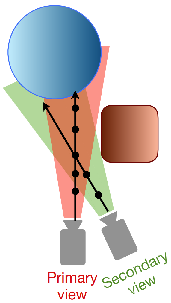
The Visibility Prior Concept

Key Insight: When given sparse input views, it is easier to estimate whether a pixel is visible in another view (relative depth) than to estimate its absolute depth accurately.

For any pixel $q$ in a primary view, the visibility prior $\tau'(q) \in \{0, 1\}$ indicates whether that pixel is also visible in a secondary view:

• $\tau'(q) = 1$: pixel is visible in both views (no occlusion)
• $\tau'(q) = 0$: pixel is occluded in the secondary view

This visibility information relates to the relative depth of scene objects - foreground objects are typically visible in multiple views, while background objects may be partially occluded.

Computing Visibility Prior using Plane Sweep Volumes

ViP-NeRF estimates the visibility prior using plane sweep volumes (PSV) without requiring any pre-training:

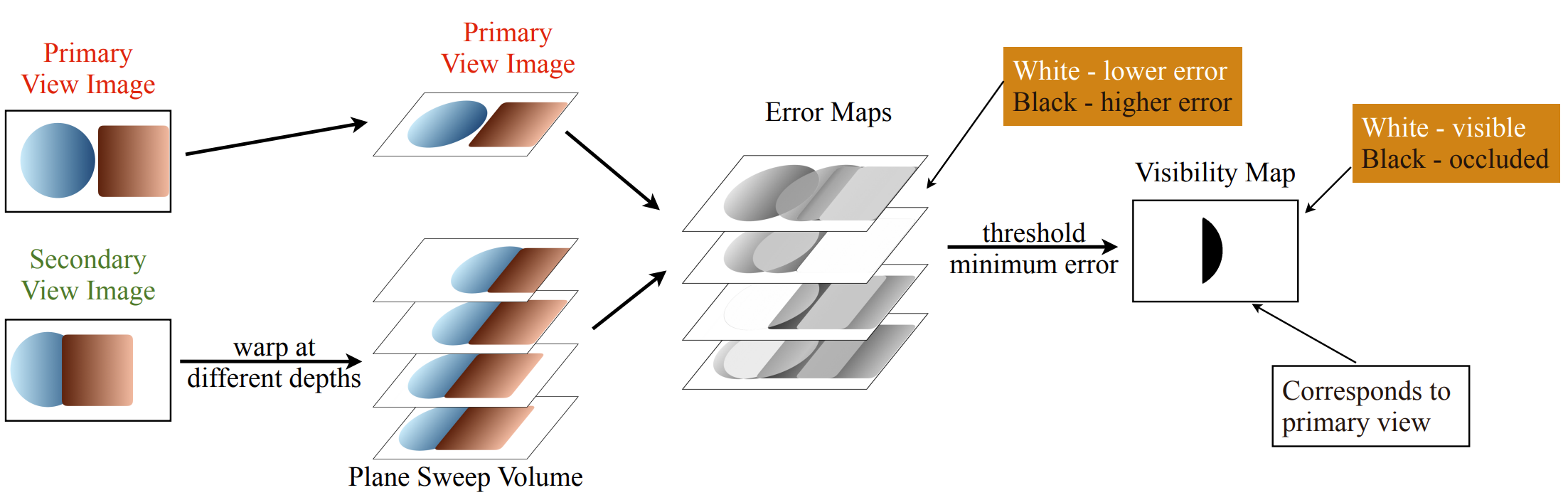
Step-by-step Process:

1. Create Plane Sweep Volume: Warp the secondary view image to the primary view at $D$ uniformly sampled depths between $z_{\min}$ and $z_{\max}$:

   • $I^{(1)}$: primary view image
   • $I^{(2)}_k$: warped secondary view images at plane $k \in \{0, 1, ..., D-1\}$

2. Compute Error Maps: For each plane $k$, calculate the L1 error:

   $$E_k = \|I^{(1)} - I^{(2)}_k\|_1$$

3. Determine Visibility: Extract the minimum error across all planes and threshold:

   $$e(q) = \min_k E_k(q)$$$$\tau'(q) = \mathbb{1}_{\{\exp(-e(q)/\gamma) > 0.5\}}$$

   where $\gamma$ is a hyperparameter (typically set to 10).

Intuition: A low error at any plane indicates a matching pixel exists in the secondary view (pixel is visible). High error across all planes suggests occlusion or highly specular surfaces. The visibility prior is only used for pixels where a match is found, avoiding unreliable regions.

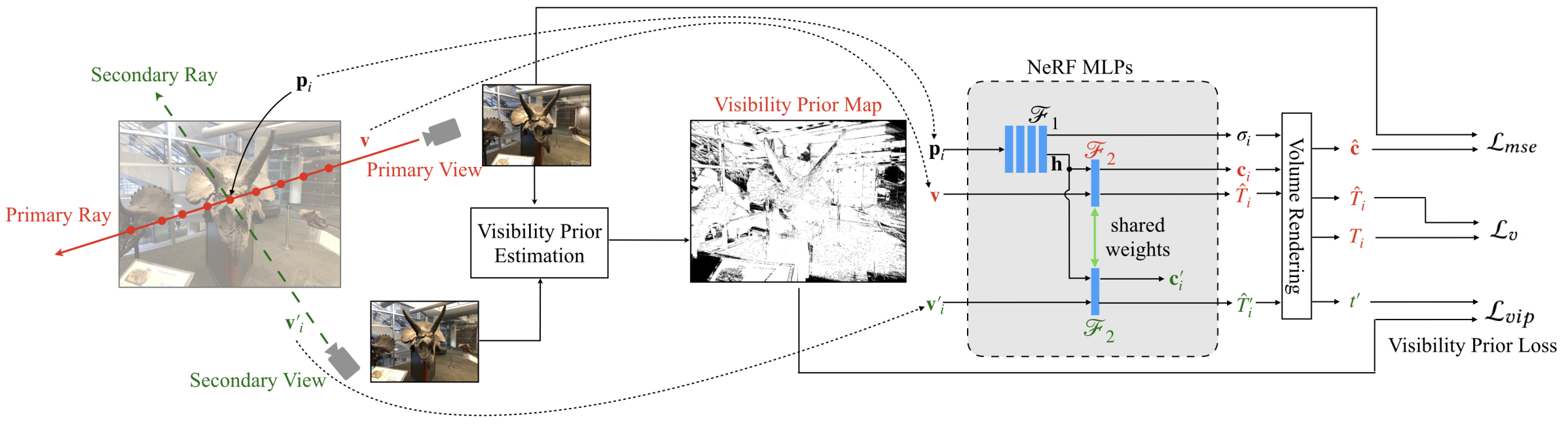
Visibility Regularization Loss

For a randomly selected pixel $q$ in the primary view, ViP-NeRF samples $N$ candidate 3D points $p_1, p_2, ..., p_N$ along the ray. The visibility of pixel $q$ in the secondary view is computed as:

$$t'(q) = \sum_{i=1}^{N} w_i T'_i \in [0,1]$$

where:

• $w_i = T_i(1 - \exp(-\delta_i \sigma_i))$ is the rendering weight from Equation (4)
• $T'_i$ is the visibility (transmittance) of point $p_i$ from the secondary view

The visibility prior loss constrains the predicted visibility to match the prior:

$$\mathcal{L}_{\text{vip}}(q) = \max(\tau'(q) - t'(q), 0)$$

This loss is only applied when $\tau'(q) = 1$ (pixel is reliably visible), avoiding supervision on uncertain occluded regions.

Efficient Visibility Prediction

Computing $T'_i$ naively requires sampling up to $N$ additional points along a secondary ray from the secondary camera to $p_i$, requiring $N^2$ MLP queries per pixel - computationally prohibitive.

Solution: Reformulate the NeRF MLP $\mathcal{F}_2$ to directly output view-dependent visibility:

$$c_i, \hat{T}_i = \mathcal{F}_2(h_i, v); \quad c'_i, \hat{T}'_i = \mathcal{F}_2(h_i, v'_i)$$

where:

• $h_i$ is the latent representation from $\mathcal{F}_1(p_i)$ (reused)
• $v$ is the primary viewing direction
• $v'_i$ is the secondary viewing direction
• $\hat{T}'_i$ is the predicted visibility in the secondary view

This reduces complexity from $N^2$ to just $N$ MLP $\mathcal{F}_1$ queries, since $\mathcal{F}_2$ is a single-layer MLP and significantly smaller.

Consistency Loss: To ensure $\hat{T}_i$ matches the volume-rendered visibility $T_i$, an additional loss is introduced:

$$\mathcal{L}_v = \sum_{i=1}^{N} \left[ \|\text{SG}(T_i) - \hat{T}_i\|^2 + \|T_i - \text{SG}(\hat{T}_i)\|^2 \right]$$

where $\text{SG}(\cdot)$ denotes stop-gradient operation. The bidirectional loss enables:

• First term: brings $\hat{T}_i$ closer to $T_i$
• Second term: transfers updates from visibility prior back to $\mathcal{F}_1$ efficiently

Complete Loss Function

ViP-NeRF combines multiple loss terms:

$$\mathcal{L} = \lambda_1 \mathcal{L}_{\text{mse}} + \lambda_2 \mathcal{L}_{\text{sd}} + \lambda_3 \mathcal{L}_{\text{vip}} + \lambda_4 \mathcal{L}_v$$

where:

• $\mathcal{L}_{\text{mse}} = \|c - \hat{c}\|^2$: standard NeRF photometric loss
• $\mathcal{L}_{\text{sd}} = \|z - \hat{z}\|^2$: sparse depth supervision from SfM (following DS-NeRF)
• $\mathcal{L}_{\text{vip}}$: visibility prior loss (dense supervision on relative depth)
• $\mathcal{L}_v$: visibility consistency loss

Hyperparameters are set as: $\lambda_1 = 1$, $\lambda_2 = 0.1$, $\lambda_3 = 0.001$, $\lambda_4 = 0.1$.

Training Strategy:

• $\mathcal{L}_{\text{vip}}$ is imposed after 20,000 iterations to ensure $\hat{T}'_i \approx T'_i$
• Total training: 50,000 iterations with Adam optimizer
• Learning rate: $5 \times 10^{-4}$ exponentially decaying to $5 \times 10^{-6}$
• Plane sweep volume parameters: $D = 64$ planes, $\gamma = 10$

Why Visibility Over Dense Depth?

Advantages of Visibility Prior:

1. No Pre-training Required: Computed using plane sweep volumes directly from input views
2. More Reliable: Focuses on relative depth rather than absolute depth
3. Dense Supervision: Provides pixel-wise constraints across view pairs
4. Cross-view Consistency: Regularizes NeRF across pairs of views, unlike single-view regularization

Comparison with Dense Depth Priors:

• Dense depth priors (like DDP-NeRF) constrain absolute depth but may be inaccurate due to generalization errors
• Visibility prior constrains relative depth ordering, providing more freedom for NeRF to reconstruct correct 3D geometry
• Visibility is inherently easier to estimate reliably without sophisticated pre-trained networks

Complementary Supervision

ViP-NeRF uses visibility prior in conjunction with sparse depth from SfM:

• Sparse depth ($\mathcal{L}_{\text{sd}}$): Provides accurate but sparse supervision on absolute depth (at SfM keypoints)
• Dense visibility ($\mathcal{L}_{\text{vip}}$): Provides dense but relative supervision across all pixels

These two priors provide complementary information:

• Sparse depth anchors the absolute scale
• Dense visibility constrains relative geometry and prevents overfitting

Ablation studies show that removing either prior degrades performance, confirming their complementary nature.

---

MiDAS

---

DUSt3R: Geometric 3D Vision Made Easy

Overview

DUSt3R (Dense Unconstrained Stereo 3D Reconstruction) represents a paradigm shift from the traditional “SfM $\rightarrow$ MVS $\rightarrow$ Meshing” pipeline. Instead of solving for camera parameters (intrinsics/extrinsics) explicitly to then triangulate points, DUSt3R treats 3D reconstruction as a direct regression problem of dense 3D pointmaps from uncalibrated images.

The Pointmap Representation

For an image $I \in \mathbb{R}^{H \times W \times 3}$, the network outputs a Pointmap $X \in \mathbb{R}^{H \times W \times 3}$:

$$ X_{i,j} = (x, y, z) \in \mathbb{R}^3 $$

This vector represents the 3D coordinates of the pixel $(i,j)$ in the scene.

Crucially, for a pair of images $I^1$ and $I^2$, the network predicts two pointmaps $X^{1,1}$ and $X^{2,1}$ where both are expressed in the coordinate frame of the first image $I^1$. This implicitly solves the pixel matching and relative pose estimation problems simultaneously without explicit geometric constraints.

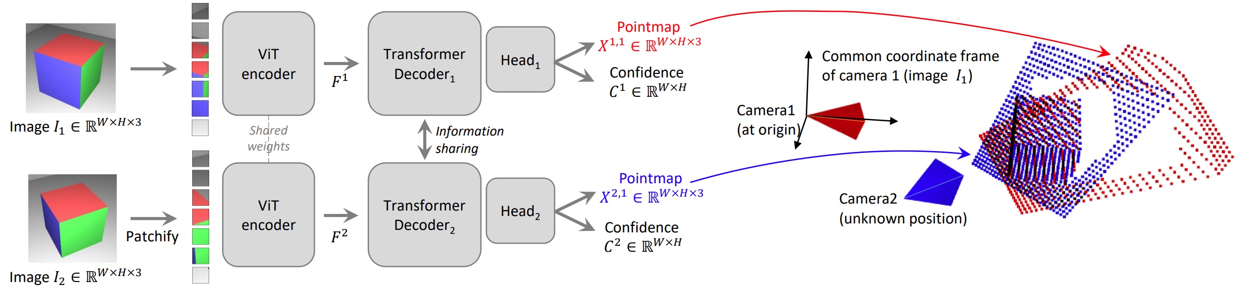
Network Architecture

The model uses a Transformer-based architecture inspired by CroCo:

1. Siamese Encoder: A shared ViT encodes $I^1$ and $I^2$ into token representations $F^1$ and $F^2$.

2. Cross-Attention Decoder: The decoder branches constantly exchange information to resolve scale and correspondences:

   $$G^1_i = \text{DecoderBlock}(G^1_{i-1}, G^2_{i-1})$$

3. Regression Heads: Outputs the pointmaps $X$ and a Confidence Map $C$ (which learns to identify invalid regions like sky or translucent objects). The confidence is defined as $C^{v,1}_i = 1 + \exp(g^{C^{v,1}_i}) > 1$, ensuring strictly positive values.

Training Objective

The network is trained with a simple 3D regression loss:

$$ \mathcal{L}_{\text{regr}}(v, i) = \frac{1}{z} X^{v,1}_i - \frac{1}{\bar{z}} \bar{X}^{v,1}_i $$

where $z$ and $\bar{z}$ are normalization factors representing the average distance of all valid points to the origin:

$$ \text{norm}(X^1, X^2) = \frac{1}{|D^1| + |D^2|} \sum_{v \in \{1,2\}} \sum_{i \in D^v} \|X^v_i\| $$

This makes the reconstruction scale-invariant.

A confidence-aware loss is also used:

$$ \mathcal{L}_{\text{conf}} = \sum_{v \in \{1,2\}} \sum_{i \in D^v} C^{v,1}_i \cdot \mathcal{L}_{\text{regr}}(v, i) - \alpha \log C^{v,1}_i $$

where $\alpha$ is a hyperparameter controlling the regularization term, encouraging the network to extrapolate in harder areas.

Global Alignment

Since the network operates pairwise, reconstructing a full scene requires fusing predictions from multiple pairs. DUSt3R constructs a connectivity graph $\mathcal{G}(\mathcal{V}, \mathcal{E})$ where vertices are images and edges indicate shared visual content between image pairs.

We seek global pointmaps $\chi$ and rigid transformations $P_e$ (pose) and $\sigma_e$ (scale) for each edge to align the pairwise predictions into a common frame:

$$ \chi^* = \mathop{\arg \min}_{\chi, P, \sigma} \sum_{e \in \mathcal{E}} \sum_{v \in e} \sum_{i=1}^{HW} C_i^{v,e} \left\| \chi_i^v - \sigma_e P_e X_i^{v,e} \right\| $$

To avoid the trivial optimum where $\sigma_e = 0, \forall e \in \mathcal{E}$, the constraint $\prod_e \sigma_e = 1$ is enforced.

This optimization aligns all pairwise pointmaps in 3D space directly, avoiding the complexity of traditional Bundle Adjustment or 2D reprojection errors. The optimization is fast and simple, typically converging in a few hundred steps using standard gradient descent.

Downstream Applications

From the predicted pointmaps, various geometric quantities can be straightforwardly extracted:

• Point Matching: Correspondences between pixels are found via reciprocal nearest neighbor search in 3D pointmap space: $\mathcal{M}^{1,2} = \{(i, j) | i = \text{NN}^{1,2}_1(j) \text{ and } j = \text{NN}^{2,1}_1(i)\}$

• Camera Intrinsics: Recovered by solving for focal length $f^*_1$ using confidence-weighted optimization. The principal point is assumed to be approximately centered.

• Relative Pose: Estimated via Procrustes alignment between pointmaps $X^{1,1} \leftrightarrow X^{1,2}$ or using PnP-RANSAC for more robustness against noise and outliers.

• Absolute Pose: Visual localization achieved by obtaining 2D-3D correspondences between query and reference images, then running PnP-RANSAC, or by estimating relative pose and scaling appropriately.

---

InstantSplat: Sparse-view 3D Reconstruction in Seconds

Overview

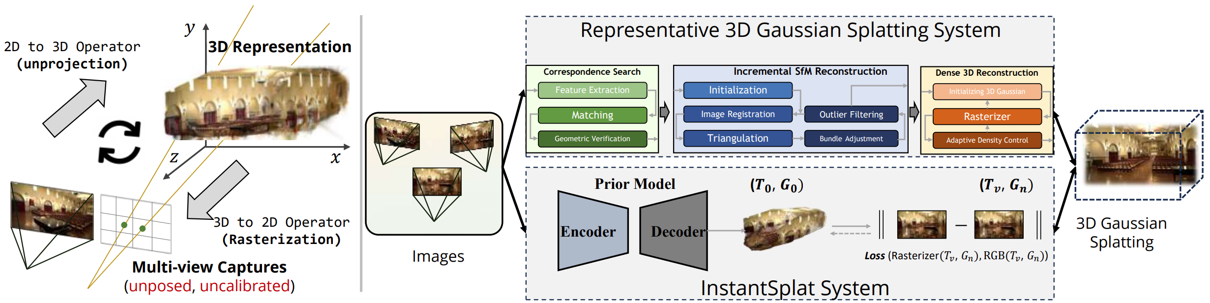
InstantSplat achieves sparse-view 3D reconstruction in seconds by removing the reliance on COLMAP SfM, which is slow and often fragile in sparse settings. It synergizes a geometric foundation model (MASt3R) for dense initialization with a fast 3DGS-based joint optimization.

The Problem with Traditional Approaches

Standard 3D-GS relies on COLMAP for:

1. Camera pose estimation
2. Sparse point cloud initialization via Structure-from-Motion

However, COLMAP is:

• Slow: Takes minutes to hours for pose estimation
• Fragile: Often fails with sparse views due to insufficient feature matches
• Error-prone: Small perturbations in poses or point distribution significantly degrade 3D-GS quality

Co-visible Global Geometry Initialization

Instead of starting from a sparse SfM cloud, InstantSplat initializes using MASt3R (a stereo prior model based on DUSt3R). This provides:

1. Dense Point Cloud: Millions of initial points derived directly from image pixels.
2. Initial Poses: Extracted from the aligned pointmaps.

View Ranking by Confidence:

Before redundancy elimination, views are ranked by their average confidence score:

$$ s_i = \frac{1}{|O^i|} \sum_{o \in O^i} o $$

where $s_i$ represents the average confidence of view $i$. Views with higher confidence are considered more reliable.

Redundancy Elimination:

Since MASt3R predicts a pointmap for every image pair, simply merging them creates massive redundancy (millions of duplicate points). InstantSplat uses a Co-visibility check, processing views in ascending order of confidence (from lowest to highest).

For each view $j$, points from higher-confidence views $\{i | s_i > s_j\}$ are projected onto view $j$:

$$ D_{\text{proj},j} = \bigcap_{\{i|s_i > s_j\}} \text{Proj}_j(\tilde{P}^i) $$

Points in view $j$ are pruned based on depth consistency:

$$ \mathcal{M}_j = \begin{cases} 1 & \text{if } |D_{\text{proj}, j} - D_{\text{orig}, j}| < \theta \\ 0 & \text{otherwise} \end{cases} $$

The final pruned pointmap is: $\tilde{P}^j = (1 - \mathcal{M}_j) \cdot \tilde{P}^j$

This significantly reduces the number of primitives and accelerates training.

Focal Length Averaging:

After global alignment, focal lengths from pairwise predictions remain inconsistent. Assuming a single-camera capture setup, InstantSplat stabilizes estimates by averaging:

$$ \bar{f} = \frac{1}{N} \sum_{i=1}^{N} f^*_i $$

This simple step significantly improves visual quality.

Joint Optimization

With the scene initialized, InstantSplat performs a Gaussian-based Bundle Adjustment. It jointly optimizes the Gaussian parameters $G$ and the camera poses $T$ by minimizing the photometric error between rendered and observed images:

$$ G^*, T^* = \mathop{\arg \min}_{G, T} \sum_{v} \left\| \hat{C}_v - \text{Rasterizer}(G, T) \right\| $$

Confidence-aware Optimizer:

To handle errors from the initialization, the learning rate for each Gaussian is dynamically scaled based on the confidence score $O_{\text{init}}$ provided by the foundation model:

$$ \text{LR}_{\text{scale}} = (1 - \text{sigmoid}(O_{\text{init}})) \cdot \beta $$

Low-confidence points (e.g., sky, reflections) have higher learning rates to allow them to be corrected rapidly, while high-confidence points maintain stable learning rates.

Pruning Strategy:

During optimization, Gaussians are removed based on:

• Opacity threshold: Gaussians with $\alpha < \epsilon$ are pruned
• World-space size: Excessively large Gaussians that likely represent floaters are removed

Test View Alignment:

For novel test views, the 3D model is frozen and only camera poses are optimized. This is done by minimizing photometric error between synthesized and actual test images, similar to iNeRF.

This approach allows InstantSplat to reconstruct scenes in $\approx 7.5$ seconds with pose accuracy superior to traditional COLMAP-free methods.

---

FSGS: Real-Time Few-shot View Synthesis

Overview

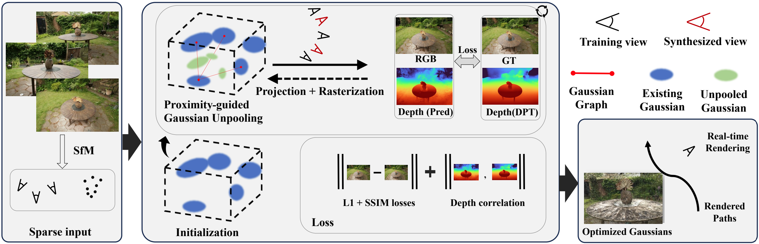
Standard 3DGS relies heavily on the density of the initial Point Cloud (from SfM/COLMAP). In few-shot scenarios (e.g., 3 views), SfM produces extremely sparse points. This leads to the optimization satisfying training views by placing “floaters” close to the camera rather than learning correct geometry, resulting in overfitting and poor novel view synthesis.

FSGS introduces a Proximity-guided Gaussian Unpooling to densify the initialization and uses Pseudo-view Depth Priors to constrain the geometry.

Proximity-guided Gaussian Unpooling

To address the limited 3D scene coverage, FSGS constructs a directed graph (the “proximity graph”) connecting each existing Gaussian $G_i$ to its $K$ nearest neighbors (typically $K=3$).

Proximity Score Calculation:

For each Gaussian $G_i$, the $K$ nearest neighbors are identified:

$$ D^K_i = \text{K-min}(d_{ij}), \quad \forall j \neq i $$

where $d_{ij} = \|\mu_i - \mu_j\|$ is the Euclidean distance between Gaussian centers.

The Proximity Score $P_i$ is calculated as the average distance to these neighbors:

$$ P_i = \frac{1}{K} \sum_{j=1}^{K} D^K_i $$

Gaussian Unpooling Strategy:

If $P_i$ exceeds a threshold $t_{\text{prox}}$, the region is considered under-reconstructed. New Gaussians are “unpooled” at the center of each edge connecting the source Gaussian to its $K$ destination neighbors.

For each new Gaussian:

• Position: Placed at the midpoint between source and destination: $\mu_{\text{new}} = \frac{\mu_{\text{source}} + \mu_{\text{dest}}}{2}$
• Scale & Opacity: Copied from the destination Gaussian
• Rotation: Initialized to identity (zero quaternion)
• SH Coefficients: Initialized to zero

This strategy encourages Gaussians to grow in representative locations and progressively fill observation gaps. The proximity graph is updated after each densification or pruning operation.

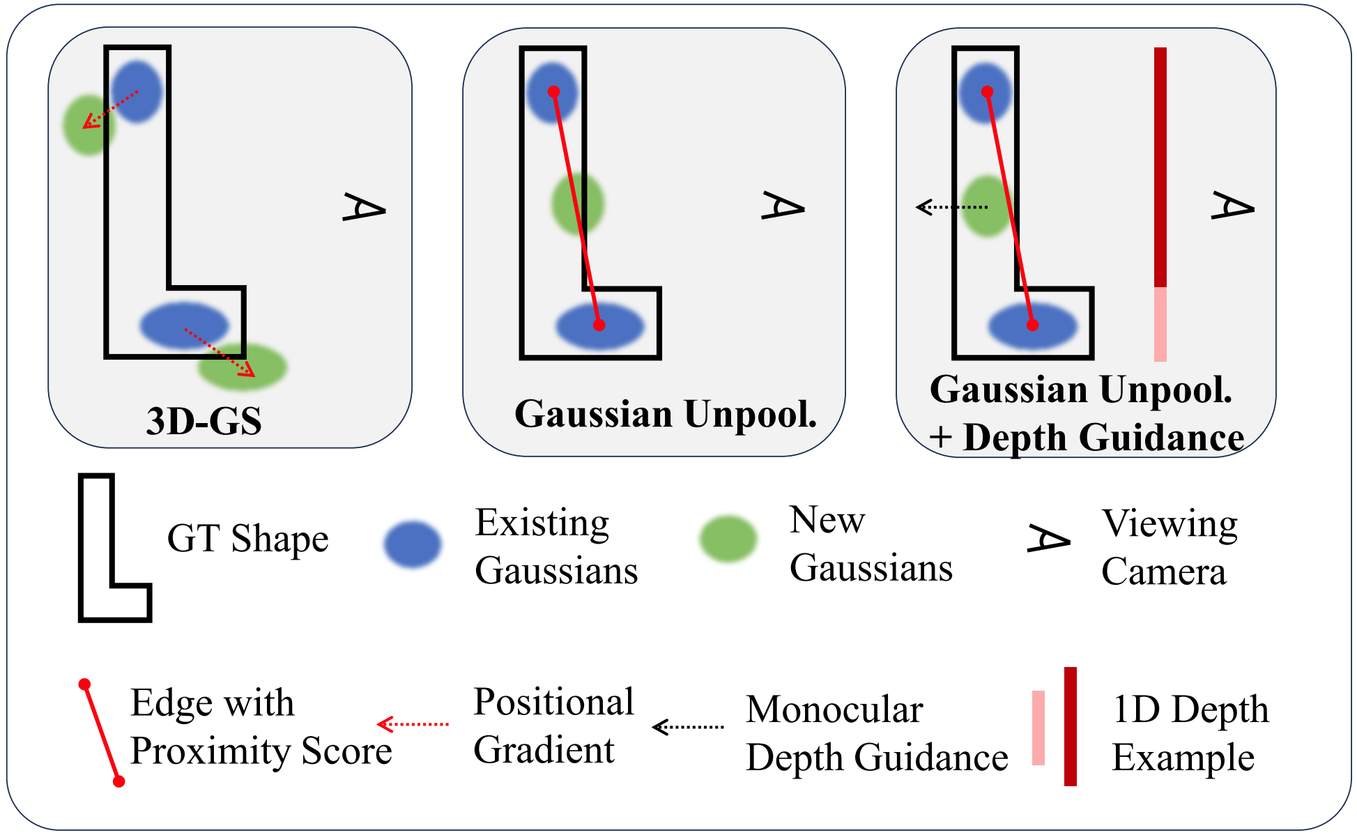
Pseudo-view & Depth Regularization

To prevent overfitting to the few training views, FSGS synthesizes Pseudo-views $P'$ by interpolating between the two closest training cameras in Euclidean space.

Pseudo-view Sampling:

$$ P' = (t + \epsilon, q), \quad \epsilon \sim \mathcal{N}(0, \delta) $$

where:

• $t$ is the camera position from a training view
• $q$ is the rotation quaternion averaged from the two nearest cameras
• $\epsilon$ adds random noise to the 3-DoF camera location

Pseudo-view sampling begins after initial convergence (typically after 2000 iterations) to ensure Gaussians roughly represent the scene first.

Differentiable Depth Rasterization:

To enable backpropagation from depth priors, FSGS implements differentiable depth rendering using alpha-blending:

$$ d = \sum_{i=1}^{n} d_i \alpha_i \prod_{j=1}^{i-1}(1 - \alpha_j) $$

where $d_i$ represents the z-buffer (depth) of the $i$-th Gaussian and $\alpha$ is identical to that in color rendering.

Pearson Correlation Loss:

Because monocular depth estimators (e.g., DPT) provide relative depth that is scale and shift invariant, FSGS uses Pearson correlation to measure depth structure alignment:

$$ \text{Corr}(\hat{D}_{\text{ras}}, \hat{D}_{\text{est}}) = \frac{\text{Cov}(\hat{D}_{\text{ras}}, \hat{D}_{\text{est}})}{\sqrt{\text{Var}(\hat{D}_{\text{ras}})\text{Var}(\hat{D}_{\text{est}})}} $$

This relaxed loss aligns the depth structure without requiring absolute depth values.

Complete Loss Function:

$$ \mathcal{L} = \lambda_1 \|C - \hat{C}\|_1 + \lambda_2 \text{D-SSIM}(C, \hat{C}) + \lambda_3 \|\text{Corr}(D_{\text{ras}}, D_{\text{est}})\|_1 $$

where $\lambda_1 = 0.8$, $\lambda_2 = 0.2$, and $\lambda_3 = 0.05$. This loss is applied to both training views and synthesized pseudo-views.

Optimization Strategy

Spherical Harmonic Progression:

Training starts with SH degree 0 (basic lighting), incrementing by 1 every 500 iterations up to degree 4. This progressive approach allows the model to first capture basic appearance before adding view-dependent effects.

Opacity Reset:

At specific iterations (e.g., 2000, 5000, 7000), opacity for all Gaussians is reset to a small value (0.05) to eliminate low-opacity floaters that don’t contribute meaningfully to the scene.

Densification Schedule:

Gaussian unpooling occurs every 100 iterations, starting after iteration 500, allowing the model to first stabilize before adding complexity.

---

Algorithm: The training pipeline of FSGS

---

1:	Training view images $\mathcal{I} = \{ I_i \in \mathbb{R}^{H \times W \times 3} \}_{i=1}^N$ and their associated camera poses $\mathcal{P} = \{ \phi_i \in \mathbb{R}^{3 \times 4} \}_{i=1}^N$.
2:	Run SfM with the input images and camera poses and obtain an initial point cloud $\mathcal{P}$, used to define 3D Gaussians function $\mathcal{G} = \{ G_i(\mu_i, \sigma_i, c_i, \alpha_i) \}_{i=1}^K$.
3:	Leverage pretrained depth estimator $\mathcal{E}$ to predict the depth map $D_i = \mathcal{E}(I_i)$.
4:	Synthesize pseudo views $\mathcal{P}^\dagger = \{ \phi_i^\dagger \in \mathbb{R}^{3 \times 4} \}_{i=1}^M$ from input camera poses $\mathcal{P}$.
5:	while until convergence do
6:	Randomly sample an image $I_i \in \mathcal{I}$ and the corresponding camera pose $\phi_i$
7:	Rasterize the rgb image $\hat{I}_i$ and the depth map $\hat{D}_i$ with camera pose $\phi_i$
8:	$\mathcal{L} = \lambda_1 \lVert I_i - \hat{I}_i \rVert_1 + \lambda_2\, \mathrm{D\!-\!SSIM}(I_i,\hat{I}_i) + \lambda_3\, \mathrm{Pearson}(D_i, \hat{D}_i)$
9:	if iteration $> t_{\text{iter}}$ then
10:	Sample a pseudo camera pose $\phi_j^\dagger \in \mathcal{P}^\dagger$
11:	Rasterize the rgb image $\hat{I}_j^\dagger$ and the depth $\hat{D}_i^\dagger$
12:	Compute the estimated depth as $D_j^\dagger = \mathcal{E}(\hat{I}_j^\dagger)$
13:	$\mathcal{L} \leftarrow \mathcal{L} + \lambda_4\, \mathrm{Pearson}(D_j^\dagger, \hat{D}_i^\dagger)$
14:	end if
15:	if IsRefinement(iteration) then
16:	for each Gaussian $G_i(\mu_i,\sigma_i,c_i,\alpha_i)$
17:	if $\alpha_i < \varepsilon$ or IsTooLarge$(\mu_i,\sigma_i)$ RemoveGaussian()
18:	if $\nabla_p \mathcal{L} > \tau_{\text{pos}}$ GaussianDensify()
19:	if NoProximity$(\mathcal{G})$ GaussianUnpooling()
20:	end for
21:	end if
22:	Update Gaussians parameter $\mathcal{G}$ via $\nabla_{\mathcal{G}} \mathcal{L}$.
23:	end while

---

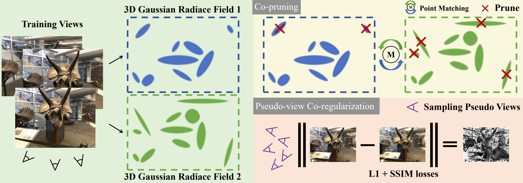
CoR-GS: Sparse-View 3D Gaussian Splatting via Co-Regularization

Overview

Two 3D Gaussian radiance fields trained from the same sparse set of views can exhibit different behaviors. By training two fields simultaneously and measuring their disagreement throughout training, one can analyze the consistency of the learned geometry and appearance. Because ground-truth supervision is applied only on training views, rendering disagreement is evaluated on unseen views.

A notable pattern is that disagreement increases significantly during densification, a phase in which new Gaussians are created but placed without strong geometric constraints. This randomness can introduce geometric errors in sparse-view 3DGS.

Key Point: Both point disagreement (differences in Gaussian positions) and rendering disagreement (differences in rendered appearance or depth) are typically negatively correlated with reconstruction accuracy.

Point Disagreement

When treating the 3D positions of Gaussians in two radiance fields as point clouds, their geometric differences can be quantified using Fitness and RMSE, metrics commonly used in point-cloud registration.

• Fitness: measures the fraction of points that successfully form correspondences within a maximum distance threshold $\tau = 5$. Higher Fitness indicates better overlap.
• RMSE: computes the root mean square of distances between corresponding points, reflecting the average positional discrepancy.

---

Rendering Disagreement

Differences between radiance fields can also be evaluated in image space.

• PSNR is used to measure disagreement between rendered RGB images.
• Relative Absolute Error (absErrorRel) is used for depth-map comparison and is widely adopted for assessing depth estimation accuracy.

---

Reconstruction Quality Evaluation

Reconstruction fidelity is typically measured by comparing rendered test-view images against ground-truth images using PSNR.

For a more comprehensive assessment, ground-truth Gaussian positions and depth maps can be obtained by training a 3D Gaussian radiance field using dense multi-view data. Evaluation then includes:

• Fitness and RMSE for geometric accuracy.
• absErrorRel for depth accuracy.

Method

CoR-GS identifies and suppresses inaccurate reconstructions using point disagreement and rendering disagreement. Two 3D Gaussian radiance fields are trained in parallel:

$$ \Theta_1 = \{\theta^1_i\}, \qquad \Theta_2 = \{\theta^2_i\}. $$

Only one field is kept for inference; the other is used to detect disagreement.
The following describes the process for $\Theta_1$ (the procedure for $\Theta_2$ is identical).

---

Co-pruning

Densification may create Gaussians that are poorly aligned with scene geometry, especially under sparse-view supervision.
Co-pruning removes Gaussians whose positions disagree across the two fields.

Nearest-neighbor correspondence

$$ f(\theta^1_i) = \mathrm{KNN}(\theta^1_i, \Theta_2). $$

Non-matching mask A Gaussian is flagged if its nearest counterpart differs by more than $\tau = 5$:

$$ M_i = \begin{cases} 1, & \sqrt{ (\theta^1_{xi} - f(\theta^1_i)_x)^2 + (\theta^1_{yi} - f(\theta^1_i)_y)^2 + (\theta^1_{zi} - f(\theta^1_i)_z)^2 } > \tau,\\[4pt] 0, & \text{otherwise}. \end{cases} $$

Pruning All Gaussians with $M_i = 1$ are removed.
Co-pruning is performed every few (e.g., 5) optimization/density-control interleaves.

---

Pseudo-view Co-regularization

Sampling pseudo-views

Pseudo-views are sampled using nearby training cameras:

$$ P' = (t + \epsilon,\, q), $$

where $t$ is a training camera position, $\epsilon \sim \mathcal{N}(0,\sigma^2)$,
and $q$ is an averaged quaternion from the two nearest cameras.

Color co-regularization

Render $I'^1$ and $I'^2$ from $\Theta_1$ and $\Theta_2$ at the pseudo-view, and enforce consistency:

$$ \mathcal{R}_{pcolor}= (1-\lambda)\,\mathcal{L}_1(I'^1, I'^2)+ \lambda\,\mathcal{L}_{\mathrm{D\text{-}SSIM}}(I'^1, I'^2). $$

Ground-truth supervision

At training views:

$$ \mathcal{L}_{color}= (1-\lambda)\,\mathcal{L}_1(I^1, I^*)+ \lambda\,\mathcal{L}_{\mathrm{D\text{-}SSIM}}(I^1, I^*). $$

Final loss

$$ \mathcal{L}= \mathcal{L}_{color}+ \lambda_p \mathcal{R}_{pcolor}, \qquad \lambda_p = 1.0. $$

---

Dynamic Scenes

Optical Flow

Overview

Given a video, optical flow is defined as a $2D$ vector field describing the apparent movement of each pixel due to relative motion between the camera (observer) and the scene (objects, surfaces, edges). The camera or the scene or both may be moving

Computing Optical Flow

We define a video as an ordered sequence of frames captured over time. $I(x, y, t)$, a function of both space and time, represents the intensity of pixel $(x, y)$ in the frame at time t. In dense optical flow, at every time t and for every pixel $(x, y)$, we want to compute the apparent velocity of the pixel in both the $x$-axis and $y$-axis, given by

$$ u(x, y, t) = \frac{\Delta x}{\Delta t}$$

$$ v(x, y, t) = \frac{\Delta y}{\Delta t}$$

The optical flow vector for each pixel is then given as $\mathbf{u} = [u, v]^{\top}$ .

Brightness constancy assumption

From the brightness constancy assumption, we can assume that the apparent intensity in the image plane for the same object does not change across different frames. We can define this as for a pixel that moved $\Delta x$ and $\Delta y$ in the $x$ and $y$ directions between times $t$ to $t + \Delta t$.

$$I(x, y, t) = I(x + \Delta x, y + \Delta y, t + \Delta t) $$

One common simplification is to use $\Delta t = 1$ (consecutive frames), such that the velocities are equivalent to the displacements $u = \Delta x$ and $v = \Delta y$ so can then obtain $I(x, y, t) = I(x + u, y + u, t + 1)$.

Small motion assumption

We assume the motion $(\Delta t, \Delta y)$ is small from frame to frame. This allows us to linearize $I$ with a first-order Taylor series expansion as:

$$ \begin{aligned} I(x+\Delta x,\, y+\Delta y,\, t+\Delta t) &= I(x,y,t)+ \frac{\partial I}{\partial x}\,\Delta x+ \frac{\partial I}{\partial y}\,\Delta y+ \frac{\partial I}{\partial t}\,\Delta t+ \ldots \\[6pt] &\approx I(x,y,t)+ \frac{\partial I}{\partial x}\,\Delta x+ \frac{\partial I}{\partial y}\,\Delta y+ \frac{\partial I}{\partial t}\,\Delta t. \end{aligned} $$

The $\dots$ represents the higher-order terms in the Taylor series expansion which we subsequently truncate out in the next line. Substituting the result into the brightness constancy assumption, we arrive at the optical flow constraint equation:

$$ \begin{aligned} 0 &= \frac{\partial I}{\partial x}\,\Delta x + \frac{\partial I}{\partial y}\,\Delta y+ \frac{\partial I}{\partial t}\,\Delta t \\[6pt] &= \frac{\partial I}{\partial x}\,\frac{\Delta x}{\Delta t}+ \frac{\partial I}{\partial y}\,\frac{\Delta y}{\Delta t}+ \frac{\partial I}{\partial t} \\[6pt] &= I_x\,u + I_y\,v + I_t \end{aligned} $$

Here, $I_x$, $I_y$, and $I_t$ denote spatial and temporal derivatives, and $u = \frac{\Delta x}{\Delta t}$, $v = \frac{\Delta y}{\Delta t}$ are the optical flow components.

$$ -I_t = I_x u + I_y v = \nabla I^\top \mathbf{u} = \nabla I \cdot \vec{\mathbf{u}}, $$

where $\nabla I = (I_x, I_y)$ and $\mathbf{u} = (u, v)$.

We recognize this as a linear system in the form of $A x = b$.
The spatial image gradient is

$$ \nabla I = \begin{bmatrix} I_x \\[4pt] I_y \end{bmatrix} \in \mathbb{R}^{2\times 1}, $$

and the unknown optical flow vector is

$$ \mathbf{u} = \begin{bmatrix} u \\[4pt] v \end{bmatrix} \in \mathbb{R}^{2\times 1}. $$

However, since $\nabla I$ is a fat matrix in the equation

$$ I_x u + I_y v = -I_t, $$

the system is under-constrained: one equation with two unknowns. Thus, the brightness constancy constraint reduces the degrees of freedom from two to one, leaving infinitely many $(u, v)$ pairs that satisfy the equation.

Lucas–Kanade (“constant” flow)

Contraint: Flow over a small patch should be the same

Assume that the surrounding patch (e.g., a $5\times5$ window) has constant flow.
Then each pixel $p_i$ in the patch contributes one optical flow constraint:

$$ I_x(p_i)\,u \;+\; I_y(p_i)\,v \;=\; -I_t(p_i), \qquad i = 1,\dots,25. $$

This gives 25 equations for the two unknowns $u$ and $v$.

In matrix form:

$$ \begin{bmatrix} I_x(p_1) & I_y(p_1) \\ I_x(p_2) & I_y(p_2) \\ \vdots & \vdots \\ I_x(p_{25}) & I_y(p_{25}) \end{bmatrix} \begin{bmatrix} u \\ v \end{bmatrix}=- \begin{bmatrix} I_t(p_1) \\ I_t(p_2) \\ \vdots \\ I_t(p_{25}) \end{bmatrix}. $$

Or compactly:

$$ A\,\mathbf{u} = \mathbf{b}, $$

where

• $A\in\mathbb{R}^{25\times 2}$ contains spatial gradients $(I_x, I_y)$,
• $\mathbf{u}\in\mathbb{R}^{2\times 1}$ is the optical flow vector,
• $\mathbf{b}\in\mathbb{R}^{25\times 1}$ contains the temporal derivatives $-I_t$.

This overdetermined system is solved in the least-squares sense:

$$ \mathbf{u} = (A^\top A)^{-1} A^\top \mathbf{b}. $$

The normal equations for Lucas–Kanade come from the matrix

$$ A^TA = \begin{bmatrix} \displaystyle \sum_{p \in P} I_x^2 & \displaystyle \sum_{p \in P} I_x I_y \\[10pt] \displaystyle \sum_{p \in P} I_y I_x & \displaystyle \sum_{p \in P} I_y^2 \end{bmatrix}. $$

Harris Corner Detector!

The Harris matrix (also called the second-moment or structure tensor) which is exactly the same matrix that appears in the Lucas–Kanade optical flow formulation.

Implications

• Corners are when $\lambda_1$, $\lambda_2$ are big; this is also when Lucas-Kanade optical flow works best
• Corners are regions with two different directions of gradient (at least)
• Corners are good places to compute flow

Problem

What happens if the image patch contains only a line? We recover the $v$ of the optical flow but not the $u$. This is the aperture problem. Want patches with different gradients to the avoid aperture problem

Horn-Schunck (“smooth” flow)

Contraint: Flow of neighboring pixels should be smooth

The optical flow has the following objective funcitons

Brightness Constance Assumption

$$ E_d(i, j)=\left( I_x\,u_{ij} + I_y\,v_{ij} + I_t \right)^2 $$

Smooth Motion Assumption

$$ E_s(i, j) = \frac{1}{4} \left[ (u_{ij} - u_{i+1,j})^2 + (u_{ij} - u_{i,j+1})^2 + (v_{ij} - v_{i+1,j})^2 + (v_{ij} - v_{i,j+1})^2 \right] $$

In Horn-Schunck optical flow we do the following:

$$\min_{u, v}\sum_{ij}\left[ E_d(i, j) + \lambda E_s(i, j) \right]$$

We can compute partial derivative, derive update equations (gradient decent)

NSFF

RAFT

RAFT DERF

4DGS

All the dynamic NeRF algorithms can be formulated as:

c, σ = M(x, d, t, λ)

where M is a mapping that maps 8D space (x, d, t, λ) to 4D space (c, σ). x reveals to the spatial point, and λ is the optional input as used to build topological and appearance changes, and d stands for view-dependency.

all the deformation NeRF based methods estimate the world-to-canonical mapping by a deformation network ϕt : (x, t) → ∆x. Then a network is introduced to compute volume density and view-dependent RGB color from each ray. The formula for rendering can be expressed as: c, σ = NeRF(x + ∆x, d, λ), λ is a frame-dependent code to model the topological and appearance change

Overview

compute the canonical-to-world mapping directly at time t using a Gaussian deformation field network F, and differential splatting follows. This enables the capability of computing backward flow and tracking for 3D Gaussians

Method

given a view matrix M = [R, T], timestamp t, our 4D Gaussian splatting framework includes 3D Gaussians G and Gaussian deformation field network F. Then a novel-view image ˆI is rendered by differential splatting [63] S following ˆI = S(M, G ′ ), where G ′ = ∆G + G.

Specifically, the deformation of 3D Gaussians ∆G is introduced by the Gaussian deformation field network ∆G = F(G, t), in which the spatial-temporal structure encoder H can encode both the temporal and spatial features of 3D Gaussians fd = H(G, t). And the multi-head Gaussian deformation decoder D can decode the features and predict each 3D Gaussian’s deformation ∆G = D(f), then the deformed 3D Gaussians G ′ can be introduced.

Spatial-Temporal Structure Encoder

Dynamic NeRFs with Deformation Fields

---

Feedforward and BARF

Pixel Splat

Overview

For every pixel feature $F[u]$ in the input feature map, a neural network $f$ predicts Gaussian primitive parameters $\Sigma$ and $S$. Gaussian locations $\mu$ and opacities $\alpha$ are not predicted directly, since this would lead to local minima.

Instead, $f$ predicts per-pixel discrete probability distributions over depths $p_{\phi}(z)$ parameterized by $\phi$. Sampling from this distribution yields the locations of the Gaussian primitives The opacity of each Gaussian is set to the probability of the sampled depth bucket. The final set of Gaussian primitives can then be rendered from novel views using the splatting algorithm. For brevity, we use $h$ to represent the function that computes depths from bucket indices.

---

BARF

This post or widget may be updated further - more notes, findings, and background will appear here!

References

1. Zhou, T., Tucker, R., Flynn, J., Fyffe, G., & Snavely, N. (2018). Stereo Magnification: High-Resolution View Synthesis. SIGGRAPH 2018.

2. Mildenhall, B., Srinivasan, P. P., Tancik, M., Barron, J. T., Ramamoorthi, R., & Ng, R. (2020). NeRF: Representing Scenes as Neural Radiance Fields for View Synthesis. ECCV 2020.

3. Fridovich-Keil, S., Yu, A., Tancik, M., Chen, Q., Recht, B., & Kanazawa, A. (2022). Plenoxels: Radiance Fields without Neural Networks. CVPR 2022 (Oral).

4. Chen, A., Xu, Z., Geiger, A., Yu, J., & Su, H. (2022). TensoRF: Tensorial Radiance Fields. ECCV 2022.

5. Müller, T., Evans, A., Schied, C., & Keller, A. (2022). Instant Neural Graphics Primitives with a Multiresolution Hash Encoding. SIGGRAPH 2022.

6. Kerbl, B., Kopanas, G., Leimkühler, T., & Drettakis, G. (2023). 3D Gaussian Splatting for Real-Time Radiance Field Rendering. SIGGRAPH 2023.

7. Deng, K., Liu, A., Zhu, J.-Y., & Ramanan, D. (2022). Depth-supervised NeRF: Fewer Views and Faster Training for Free. CVPR 2022.

8. Somraj, N., & Soundararajan, R. (2023). ViP-NeRF: Visibility Prior for Sparse Input Neural Radiance Fields. SIGGRAPH 2023.

9. Ranftl, R., Bochkovskiy, A., & Koltun, V. (2021). Vision Transformers for Dense Prediction (DPT / MiDaS). ICCV 2021.

10. Wang, W., et al. (2024). DUSt3R: Geometric 3D Vision Made Easy. CVPR 2024.

11. Leroy, V., Cabon, Y., & Revaud, J. (2024). Grounding Image Matching in 3D with MASt3R. arXiv:2406.09756.

12. Fan, Z., Wang, K., Wen, K., Zhu, Z., Xu, D., Wang, Z., & others. (2024). InstantSplat: Unbounded Sparse-view Pose-free 3D Gaussian Splatting in 40 Seconds. arXiv:2403.20309.

13. Zhu, Z., Fan, Z., Jiang, Y., & Wang, Z. (2024). FSGS: Real-Time Few-Shot View Synthesis using Gaussian Splatting. ECCV 2024.

14. Zhang, J., et al. (2024). CoR-GS: Sparse-View 3D Gaussian Splatting via Co-Regularization. CVPR 2024.

15. Lucas, B. D., & Kanade, T. (1981). An Iterative Image Registration Technique with an Application to Stereo Vision. IJCAI 1981.

16. Horn, B. K. P., & Schunck, B. G. (1981). Determining Optical Flow. Artificial Intelligence, 17(1–3).

17. Teed, Z., & Deng, J. (2020). RAFT: Recurrent All-Pairs Field Transforms for Optical Flow. ECCV 2020.

18. Stanford CS231A Notes: Optical Flow. https://web.stanford.edu/class/cs231a/course_notes/09-optical-flow.pdf

19. CMU 16-385 Notes: Optical Flow. https://www.cs.cmu.edu/~16385/s15/lectures/Lecture21.pdf

20. Li, Z., Niklaus, S., Mai, L., Yang, J., & Ranjan, R. (2021). Neural Scene Flow Fields (NSFF). CVPR 2021.

21. Wu, G., et al. (2024). 4D Gaussian Splatting for Real-Time Dynamic Scene Rendering. CVPR 2024.

22. Charatan, D., Li, S., Tagliasacchi, A., & Sitzmann, V. (2024). PixelSplat: 3D Gaussian Splats from Image Pairs for Scalable Generalizable 3D Reconstruction. CVPR 2024.

23. Chen, A., Barron, J. T., Srinivasan, P. P., Xiang, T., & Ng, R. (2021). BARF: Bundle-Adjusting Neural Radiance Fields. ICCV 2021.