These notes follow the NPTEL course Computer Architecture and Organization (IIT Kharagpur) [1], with definitions and figures from Hamacher et al. [2], Stallings [3] and Hennessy & Patterson [4].
Basics of Computer Organization
Architecture and Organization
Computer organization is the design of the components and functional blocks from which a computer is built. Computer architecture is how these components are integrated into a system that achieves a desired level of performance.
Functional Units
All instructions and data are stored in memory. An instruction and the data it needs are brought into the processor and executed there, and input and output devices connect the computer to the outside world. This is the von Neumann architecture.
- Processor (CPU): a control unit and an arithmetic logic unit (ALU).
- The ALU contains registers and the circuits for arithmetic (add, subtract, multiply, divide) and logic (AND, OR, NOT, shift, compare). The operands are brought into registers, the operation is carried out, and the result is stored in a register or in memory.
- The control unit decodes the instruction’s opcode and generates the control signals in the required sequence. For $R1 \leftarrow R2 + R3$ it enables the outputs of $R2$ and $R3$, selects addition, and stores the adder output in $R1$.
- Memory: primary (main) memory holds the active program and data, and secondary memory holds all programs and data as files. The processor has direct access only to primary memory. The memory system is a hierarchy: L1, L2 and L3 caches, main memory, secondary memory.
- RAM: the access time does not depend on the location. Used for caches and main memory.
- ROM: fixed data that cannot be changed.
- Magnetic disk: the access time depends on the location. Used as secondary memory.
- Flash memory: faster than disk, and replacing it as secondary memory.
Basic Operation
The following special-purpose registers are used:
- Memory Address Register (MAR): the address of the memory location to be accessed.
- Memory Data Register (MDR): the data to be written into memory, or the data read from memory.
- Program Counter (PC): the address of the next instruction. It is incremented when an instruction is fetched.
- Instruction Register (IR): the instruction fetched from memory, while it is decoded.
- Read: load the address into MAR and issue READ. The data read is stored in MDR.
- Write: load the address into MAR and the data into MDR, then issue WRITE.
The steps carried out to execute an instruction are called micro-operations. Every instruction starts with the fetch:
$$\text{MAR} \leftarrow \text{PC}, \qquad \text{MDR} \leftarrow \text{Mem[MAR]}, \qquad \text{IR} \leftarrow \text{MDR}, \qquad \text{PC} \leftarrow \text{PC} + 4$$and the control unit then decodes IR.
ADD R1, LOCA ($R1 \leftarrow R1 + \text{Mem[LOCA]}$) is stored at address 1000, with $R1 = 50$, $\text{LOCA} = 5000$ and $\text{Mem[5000]} = 75$.
ADD R1, LOCA.| Step | Micro-operation | Result |
|---|---|---|
| 1 | $\text{MAR} \leftarrow \text{PC}$ | MAR = 1000 |
| 2 | $\text{MDR} \leftarrow \text{Mem[MAR]}$ | MDR = ADD R1, LOCA |
| 3 | $\text{IR} \leftarrow \text{MDR}$, $\text{PC} \leftarrow \text{PC} + 4$ | PC = 1004; decode |
| 4 | $\text{MAR} \leftarrow \text{IR[operand]}$ | MAR = 5000 |
| 5 | $\text{MDR} \leftarrow \text{Mem[MAR]}$ | MDR = 75 |
| 6 | $R1 \leftarrow R1 + \text{MDR}$ | R1 = 125 |
For ADD R1, R2 the fetch is the same, and after decoding there is only one step, $R1 \leftarrow R1 + R2$.
Bus Architecture
A bus is a group of lines that connects several devices.
- With a single bus, only one data transfer is possible in a clock cycle.
- With multiple buses, several transfers can be done in the same cycle, so instructions execute faster. Several short buses also have smaller parasitic capacitance, and hence smaller delay, than one long bus.
At the system level the processor, memory and I/O devices may share a single bus, or I/O may be connected through an I/O processor on a second bus. Inside the processor, the registers and the ALU can also be connected by a single internal bus:
Memory Addressing
Memory is an array of locations, each with a unique address. A memory with $M$ locations of $N$ bits is an $M \times N$ memory (e.g. $1024 \times 8$), and $n$ address bits can address $2^n$ locations. Memory is usually byte-addressable: every byte has an address, and an instruction can access a half-word (2 B), a word (4 B) or a long word (8 B). The word size depends on the machine, typically 32 or 64 bits.
(a) A computer has 64 MB of byte-addressable memory. How many address bits are needed? (b) A computer has 1 GB of memory with 32-bit words. How many bits are needed to address a word?
(a) $64\text{ MB} = 2^6 \times 2^{20} = 2^{26}$ B, so 26 bits. (b) $2^{30} / 4 = 2^{28}$ words, so 28 bits.
Byte Ordering
- Little endian: the least significant byte is stored at the lowest address (x86, including the Ryzen 7 5800H).
- Big endian: the most significant byte is stored at the lowest address (network byte order in TCP/IP).
01010101 00110011 00001111 11000011 stored from address 2000.| Address | Big endian | Little endian |
|---|---|---|
| 2000 | 01010101 | 11000011 |
| 2001 | 00110011 | 00001111 |
| 2002 | 00001111 | 00110011 |
| 2003 | 11000011 | 01010101 |
Load and Store
A load reads a memory location into a register (LOAD R1, 2000), and a store writes a register into memory (STORE 2020, R3). For example, $S = (A + B) - (C - D)$:
LOAD  R1, A
LOAD  R2, B
ADD   R3, R1, R2    // R3 = A + B
LOAD  R1, C
LOAD  R2, D
SUB   R4, R1, R2    // R4 = C - D
SUB   R3, R3, R4    // R3 = R3 - R4
STORE S, R3
Machine, Assembly and High-Level Languages
- Machine language is executed directly by the hardware; instructions are binary codes.
- Assembly language is a symbolic version of machine language, with a one-to-one correspondence to it.
- High-level languages (C, C++, Java) are closer to human languages.
An assembler translates assembly language to machine code. A compiler translates a high-level language program, either directly to machine code or first to assembly language. A cross-assembler or cross-compiler runs on one machine and generates code for another, e.g. a compiler running on a PC that generates code for a phone.
von Neumann and Harvard Architectures
- von Neumann: instructions and data are stored in the same memory. It is flexible, easy to implement, and used in most general-purpose processors. The processor–memory bus is a bottleneck, since all instructions and data pass through it.
- Harvard: instructions are stored in a program memory and data in a data memory, so an instruction fetch and a data access can be done in parallel. Used in some microcontrollers, and in pipelines with separate instruction and data caches. The processor–memory bottleneck remains.
In a pipeline, instruction execution is divided into 5 stages: IF (instruction fetch), ID (decode), EX (ALU operation), MEM (memory access) and WB (write back). In clock cycle 4, instruction 4 is in IF while instruction 1 is in MEM. With a single memory one of them has to wait; with separate memories both proceed.
Instruction Set Architecture
The instruction set architecture (ISA) is the interface between software and hardware. It consists of the programmer’s view of the machine (registers, address and data buses) and the instruction set.
Many ISAs are used across generations of machines (x86 has been extended from 16 to 64 bits and still runs on the Ryzen 7 5800H). The design issues of an instruction set are:
- the number of explicit operands (0, 1, 2 or 3);
- the location of the operands (registers, accumulator, memory) and how they are specified (addressing modes);
- the operand sizes (byte, half-word, word, double word);
- the operations (ADD, SUB, MUL, AND, OR, CMP, MOVE, JMP, …).
Types of ISA
| Type | Example | Operation |
|---|---|---|
| Stack | ADD | TOS ← TOS + NEXT |
| Accumulator | ADD X | ACC ← ACC + Mem[X] |
| Memory–memory | ADD A,B,C | Mem[A] ← Mem[B] + Mem[C] |
| Register–memory | ADD R1,X | R1 ← R1 + Mem[X] |
| Load–store | ADD R1,R2,R3 | R1 ← R2 + R3 |
In a load–store architecture only LOAD and STORE instructions access memory, and all other instructions operate on registers. This is the basis of RISC (reduced instruction set computer; see CISC and RISC below).
Write $Y = A/B - (A - C \times B)$ for each type of machine.
; stack
PUSH A
PUSH B
DIV          ; A/B
PUSH A
PUSH C
PUSH B
MUL          ; C*B
SUB          ; A - C*B
SUB          ; A/B - (A - C*B)
POP  Y
; accumulator
LOAD  C
MUL   B
STORE D      ; D = C*B
LOAD  A
SUB   D
STORE D      ; D = A - C*B
LOAD  A
DIV   B
SUB   D
STORE Y
; memory-memory (3 operands)
DIV  D, A, B   ; D = A/B
MUL  E, C, B   ; E = C*B
SUB  E, A, E   ; E = A - E
SUB  Y, D, E
; load-store
LOAD  R1, A
LOAD  R2, B
LOAD  R3, C
DIV   R4, R1, R2
MUL   R5, R3, R2
SUB   R5, R1, R5
SUB   R4, R4, R5
STORE Y, R4
Older architectures had many special-purpose registers (PC, stack pointer, index register, flags, accumulator); newer ones have many general-purpose registers (GPRs).
- It is easy for the compiler to assign variables to registers.
- Registers are much faster than memory.
- Fewer bits are needed to specify a register, so the instruction encoding is more compact.
- The drawback is that more registers must be saved and restored on procedure calls and interrupts.
Instruction Format
An instruction consists of an opcode, which specifies the operation (data transfer, arithmetic and logic, control, I/O, machine control), and operands, which specify the sources and the destination (immediate data, a register or a memory address).
- Implied:
NOP,HALT - 1-address:
ADD X,LOAD M - 2-address:
ADD X, Y - Register–memory:
ADD R1, X - Register–register:
ADD R1, R2, R3
Fixed-size instructions are easier to decode. With 32 registers a register is specified in 5 bits; for example, in a 32-bit format, LOAD R11, 100(R2) is encoded as a 6-bit opcode, two 5-bit register fields and a 16-bit immediate.
Expanding Opcodes
For a fixed instruction length there is a trade-off between the number of opcodes and the addressing capability: more opcode bits leave fewer bits for addresses. A refinement is the variable-length (expanding) opcode: there is a minimum opcode length, but for some opcodes further operations are specified using additional bits of the instruction. Since the instruction length is fixed, those instructions have fewer bits for addressing, so this is used for instructions that need fewer operands or less powerful addressing [3].
Consider 12-bit instructions with a 3-bit opcode [3].
- Opcodes 0–5 are memory-reference instructions (an address plus page and indirect bits), so there are only six basic operations.
- Opcode 6 is I/O: 6 bits select one of 64 devices and 3 bits give the command.
- Opcode 7 is a register-reference (microinstruction) format: each remaining bit specifies an operation, such as clear accumulator, and the bits can be combined.
With this opcode extension, about 35 instructions fit in 12 bits.
How Many Instructions Can Be Encoded
Each opcode pattern not used by a longer-address format becomes a prefix for the next format, which takes over the bits of the address field it no longer needs. No opcode may be a prefix of another, so the instruction can still be decoded.
With $n$-bit instructions and $k$-bit address fields, a two-address instruction has $n - 2k$ opcode bits, i.e. $2^{n-2k}$ patterns. If $T_2$ of them are used, then
$$N_1^{\max} = \left(2^{n-2k} - T_2\right) 2^k, \qquad N_0^{\max} = \left(\left(2^{n-2k} - T_2\right) 2^k - T_1\right) 2^k$$where $T_1$ is the number of one-address instructions actually used and $N_1^{\max}$, $N_0^{\max}$ are the most one- and zero-address instructions possible.
16-bit instructions and 6-bit address fields, with 15 two-address and 60 one-address instructions. How many zero-address instructions are possible?
- Two-address: $16 - 12 = 4$ opcode bits, 16 patterns. 15 are used (
0000–1110), so 1 pattern (1111) is left. - One-address:
1111plus 6 more bits gives $1 \times 2^6 = 64$ patterns. 60 are used, so 4 are left. - Zero-address: each of those 4 patterns plus the last 6 bits gives $4 \times 2^6 = 256$ instructions.
| Format | Opcode | Addresses |
|---|---|---|
| two-address | 4 bits: 0000–1110 | $A_1$ (6), $A_2$ (6) |
| one-address | 10 bits: 1111 000000–1111 111011 | $A$ (6) |
| zero-address | 16 bits: 1111 111100 xxxxxx–1111 111111 xxxxxx | none |
Addressing Modes
An addressing mode specifies how the operand of an instruction is located. The address from which the operand is finally read is the effective address (EA).
CISC (complex instruction set computer) ISAs support many addressing modes; load–store ISAs support very few.
| Mode | Example | Operand | Accesses |
|---|---|---|---|
| Immediate | ADDI R1, R2, 42 | in the instruction | 0 |
| Register | ADD R1, R2, R3 | in register R2 | 0 |
| Direct (absolute) | ADD R1, 20A6H | Mem[20A6] | 1 |
| Indirect | ADD R1, (20A6H) | Mem[Mem[20A6]] | 2 |
| Register indirect | ADD R1, (R5) | Mem[R5] | 1 |
| Indexed | LOAD R1, 1050(R3) | Mem[1050 + R3] | 1 |
| PC-relative | BEQ …, offset | target = PC + offset | — |
| Autoincrement | ADD R1, (R2)+ | Mem[R2], then R2 += size | 1 |
| Autodecrement | ADD R1, −(R2) | R2 −= size, then Mem[R2] | 1 |
- Immediate: no memory access is needed, but the range is limited by the number of bits of the constant.
- Direct: one memory access, but the address space is limited by the size of the address field.
- Indirect: two memory accesses, but a large address space.
- Register: few bits are needed and there is no memory access.
- Register indirect: a large address space, with one memory access fewer than indirect addressing.
- Indexed: the offset is the starting address of an array and the index register selects the element.
- PC-relative: the offset is added to PC, which by then usually holds the address of the next instruction. With a 12-bit offset the range is $-2048$ to $+2047$.
- Stack: the operand is on top of the stack (
PUSH X,POP X,ADD). The stack pointer (SP) is updated byPUSH,POP,CALLandRET. - Base: all addresses are added to a base (segment) register, so code and data can be moved in memory.
- Autoincrement and autodecrement: the register holding the address is incremented after the access, or decremented before it (like
a++and--ain C) [2].
CISC and RISC
Complex Instruction Set Computer (CISC):
- complex instruction set with many addressing modes (R–R, R–M, M–M, indexed, indirect, …);
- special-purpose registers and flags (sign, zero, carry, overflow);
- variable-length instructions and complex encoding;
- easy mapping of high-level language statements to machine instructions;
- complex instruction decoding and control unit, and a complex pipeline implementation.
Example: x86, including the Ryzen 7 5800H. CISC machines have had modes such as memory indirect (ADD R1, @(R4): $R1 \leftarrow R1 + \text{Mem[Mem[R4]]}$) and scaled (ADD R1, 50(R2)[R3]: $R1 \leftarrow R1 + \text{Mem}[50 + R2 + R3 \times d]$).
Reduced Instruction Set Computer (RISC), or load–store architecture:
- simple architecture for efficient pipelining;
- simple instruction set with very few addressing modes;
- many general-purpose registers and very few special-purpose ones;
- uniform instruction length and encoding, so decoding is easy;
- compiler-assisted scheduling of the pipeline.
Examples: MIPS (used in these notes), ARM (most phones).
A 1991 comparison of a CISC and a RISC machine found that the RISC machine executed about twice as many instructions, but the CPI (average cycles per instruction) of the CISC machine was about six times larger. So the RISC machine was about three times faster, and needed much less hardware. x86 remains CISC because of backward compatibility: the user sees a CISC instruction set, the hardware translates each instruction into RISC-like instructions, and these are executed in a pipeline.
MIPS32
MIPS32 is a RISC ISA. Its programmer-visible registers are:
- 32 general-purpose 32-bit registers $R0$–$R31$.
- $R0$ is hard-wired to 0. It can be the destination of an instruction whose result is discarded, or a source of zero.
- $R31$ stores the return address on a function call (
JAL,BLTZAL,BGEZAL).
- A 32-bit PC, changed only by branch and jump instructions.
- HI and LO, which hold the 64-bit product of a multiply (HI the upper 32 bits, LO the lower), and the remainder (HI) and quotient (LO) of a divide.
There is no separate stack pointer, index register or flag register. Any GPR can be used as a stack pointer or index register, and conditions are kept in registers instead of flags, which avoids problems in a pipeline.
| Name | Number | Use |
|---|---|---|
$zero | R0 | constant 0 |
$at | R1 | reserved for the assembler (pseudo-instructions) |
$v0–$v1 | R2–R3 | function results, expression evaluation |
$a0–$a3 | R4–R7 | first four function arguments |
$t0–$t9 | R8–R15, R24–R25 | temporaries, not preserved across calls |
$s0–$s7 | R16–R23 | saved temporaries, preserved across calls |
$k0–$k1 | R26–R27 | reserved for the OS kernel |
$gp | R28 | global pointer |
$sp | R29 | stack pointer |
$fp | R30 | frame pointer |
$ra | R31 | return address |
Words must be aligned: the address of a word is a multiple of 4 (the last two bits are 00), so a word can be fetched in one cycle. A misaligned word may need two cycles.
Instruction Classes
- Load and store: memory is accessed only through these.
LB,LH,LWload a byte, half-word or word (sign-extended);LBU,LHUload without sign extension;SB,SH,SWstore.LWL,LWR,SWL,SWRaccess unaligned words, andLL,SC(load linked, store conditional) do an atomic read–modify–write. - Arithmetic and logic, all on registers:
- with a 16-bit immediate:
ADDI,ADDIU,ANDI,ORI,XORI,SLTI,LUI; - with three registers:
ADD,ADDU,SUB,SUBU,AND,OR,NOR,XOR,SLT,SLTU; - shifts:
SLL,SRL,SRA(and variable versions),ROTR.
- with a 16-bit immediate:
- Multiply and divide:
MULT,MULTU,DIV,DIVUwrite HI and LO, andMFHI,MFLOread them.MULwrites the low 32 bits of the product to a GPR. - Jump and branch:
BEQandBNEcompare two registers;BGEZ,BGTZ,BLEZ,BLTZcompare with zero. These are PC-relative, with a 16-bit offset.JandJALjump within a 256 MB region;JRandJALRjump to the address in a register.
- Miscellaneous:
SYSCALL,BREAK, traps (TEQ,TGE, …), conditional moves (MOVZ,MOVN),PREF,NOP. Coprocessor instructions are for CP0 (virtual memory and exceptions) and CP1 (floating point).
Instruction Encoding
All MIPS32 instructions are 32 bits long, in one of three formats. Since fields such as rs and rt are in the same position in every format, the registers can be read and the immediate sign-extended while the opcode is being decoded, in case they are needed.
- R-type: two source registers
rs,rtand a destinationrd;shamtis the shift amount andfunctselects the ALU operation. Foradd $t1, $s1, $s2($t1= R9,$s1= R17,$s2= R18; opcode 0, funct 100000) the encoding is000000 10001 10010 01001 00000 100000. - I-type: a source
rs, a destinationrtand a 16-bit immediate. Used for loads, stores, ALU-immediate instructions and branches. Forlw $t1, 48($s1)(opcode 100011) the encoding is100011 10001 01001 0000000000110000. - J-type: a 26-bit address, shifted left by 2 to give 28 bits.
MIPS32 addressing modes:
- register:
add $s1, $s2, $s3 - immediate:
addi $s1, $s2, 200 - base (displacement):
lw $s1, 150($s2) - PC-relative:
beq $s1, $s2, Label, the 16-bit offset is added to PC - pseudo-direct:
j Label, the 26-bit field is shifted left by 2 and combined with the upper bits of PC
Programming Examples
# A[10] = X - A[12]        ($s3 = &A[0], $s2 = X; 4 bytes per element)
lw   $t0, 48($s3)          # $t0 = A[12]
sub  $t0, $s2, $t0
sw   $t0, 40($s3)          # A[10] = $t0

# if (x < y) z = x - y; else z = x + y;     ($s0 = x, $s1 = y, $s3 = z)
      slt  $t0, $s0, $s1    # $t0 = 1 if x < y
      beq  $t0, $zero, Lab1
      sub  $s3, $s0, $s1
      j    Lab2
Lab1: add  $s3, $s0, $s1
Lab2:
MIPS has only beq and bne for comparing two registers, so < is implemented with slt followed by a branch. The assembler provides pseudo-instructions, which it translates into MIPS32 instructions using $at:
| Pseudo-instruction | Translates to |
|---|---|
blt $1, $2, L | slt $at, $1, $2 ; bne $at, $zero, L |
bgt $1, $2, L | slt $at, $2, $1 ; bne $at, $zero, L |
move $1, $2 | add $1, $2, $zero |
li $1, 0x23ABCD | lui $1, 0x0023 ; ori $1, $1, 0xABCD |
About 90% of constants fit in 16 bits and need one instruction. A 32-bit constant needs two: lui loads the upper 16 bits (the lower 16 become 0), and ori inserts the lower 16 bits. For example, 0xAAAA3333 is loaded with lui $s1, 0xAAAA and ori $s1, $s1, 0x3333.
A function is called with jal Label, which jumps and stores the return address in $ra, and returns with jr $ra.
Performance Evaluation
Measuring CPU Performance
A processor runs with a clock of rate $f$, and the clock cycle time is $C = 1/f$. A machine instruction consists of micro-operations that take one cycle each, so an instruction takes one or more cycles. For a program running on a machine:
- $IC$: the instruction count (number of instructions executed);
- $CPI$: the average number of cycles per instruction;
- $C$: the clock cycle time.
Performance is the reciprocal of the execution time, so the speedup of machine $A$ over machine $B$ is
$$\text{Speedup} = \frac{\text{Perf}_A}{\text{Perf}_B} = \frac{XT_B}{XT_A}$$| $IC$ | $CPI$ | $C$ | |
|---|---|---|---|
| Program | ✓ | ✓ | |
| Compiler | ✓ | ✓ | |
| ISA | ✓ | ✓ | |
| CPU organization | ✓ | ✓ | |
| Hardware technology | ✓ |
It is difficult to change one factor without affecting the others. RISC increases $IC$ but decreases $CPI$ and $C$; CISC decreases $IC$ but increases $CPI$ and $C$. Experimentally, RISC gives better performance.
Machine A runs a program with CPI 2.3. Machine B, with the same ISA and a better compiler, runs it with 20% fewer instructions and CPI 1.7 at 1.2 GHz. What clock rate must A have for the same performance?
CPI from Instruction Classes
If there are $n$ classes of instructions, $IC_i$ instructions of class $i$ each take $CPI_i$ cycles, and $F_i = IC_i / IC$ is the frequency of class $i$, then
$$\text{CPU cycles} = \sum_{i=1}^{n} IC_i \times CPI_i, \qquad CPI = \frac{\sum_i IC_i \times CPI_i}{IC} = \sum_{i=1}^{n} F_i \times CPI_i$$Instruction types A, B and C have CPI 1.3, 2.2 and 2.0 and frequencies 60%, 10% and 30%. Which is better: reducing the CPI of A to 1.1, or that of B to 1.6?
- (a) $0.6 \times 1.1 + 0.1 \times 2.2 + 0.3 \times 2.0 = 1.48$.
- (b) $0.6 \times 1.3 + 0.1 \times 1.6 + 0.3 \times 2.0 = 1.54$.
So option (a) is better.
MIPS and MFLOPS
$$\text{MIPS} = \frac{IC}{XT \times 10^6} = \frac{\text{clock rate (MHz)}}{CPI}$$Problems with MIPS (millions of instructions per second):
- it depends on the instruction set, so it cannot compare machines with different ISAs;
- it varies between programs on the same machine;
- a higher MIPS rating does not always mean better performance. With a floating-point coprocessor, a program runs faster but executes fewer, more complex instructions, so the MIPS rating is lower; with software floating point it is slower but has a higher MIPS rating.
The MIPS rating is valid only when the same program, ISA and compiler are used, i.e. the machine code is identical.
MFLOPS (millions of floating-point operations per second) is suited to programs with many floating-point computations. But different machines implement different floating-point operations, these take different times (division is much slower than addition), and a program with no floating-point operations, such as a compiler, has an MFLOPS rating of 0.
A 1 GHz processor has instruction classes A, B, C with CPI 1, 2, 3. Two compilers produce (7, 2, 1) and (12, 1, 1) million instructions of each class. Find the MIPS rating and the CPU time for each.
- Compiler 1: $CPI = (7 + 4 + 3)/10 = 1.40$, MIPS $= 1000/1.40 = 714.3$, time $= 10 \times 10^6 \times 1.40 / 10^9 = 0.014$ s.
- Compiler 2: $CPI = (12 + 2 + 3)/14 = 1.21$, MIPS $= 1000/1.214 = 823.5$, time $= 14 \times 10^6 \times 1.21 / 10^9 = 0.017$ s.
The MIPS rating says compiler 2 is faster, but its program takes longer.
Benchmarks
A benchmark is a set of standard programs used to compare the performance of machines. Four levels of programs are used:
- Real applications: a suite of programs typical of the target workload, such as SPEC (System Performance Evaluation Corporation). SPEC CPU2006 has 12 integer (CINT2006) and 17 floating-point (CFP2006) programs.
- Kernel benchmarks: computation-intensive pieces extracted from real programs (Livermore Loops, Linpack). They are used to evaluate specific features of a machine.
- Toy benchmarks: programs of 10–100 lines (sieve of Eratosthenes, quicksort). They are easy to run but of limited use.
- Synthetic benchmarks: artificial programs that match the average frequency of operations of a large set of programs (Whetstone, Dhrystone). Compilers can inflate their results; optimizing compilers can discard over 25% of Dhrystone.
Benchmark results must be reproducible, so the hardware, software, compiler flags and tuning parameters are specified.
Summarizing Performance
| A | B | C | |
|---|---|---|---|
| P1 | 1 | 10 | 25 |
| P2 | 500 | 250 | 10 |
| Total | 501 | 260 | 35 |
A is 10 times faster than B for P1, but B is 2 times faster than A for P2. The results can be summarized as follows.
- Total (or arithmetic mean) execution time, $\frac{1}{n}\sum_i XT_i$. B is $501/260 = 1.93$ times faster than A, and C is $501/35 = 14.3$ times faster than A. This is correct only if the programs run equally often.
- Weighted arithmetic mean, $\sum_i W_i \times XT_i$, where $W_i$ is the fraction of the workload that is program $i$. With $W = (0.5, 0.5)$: A = 250.5, B = 130, C = 17.5. With $W = (0.9, 0.1)$: A = 50.9, B = 34, C = 23.5.
- Normalized execution time: each time is divided by the time on a reference machine, and the results are averaged. SPEC uses this.
| Reference | A | B | C |
|---|---|---|---|
| A: arithmetic | 1.0 | 5.25 | 12.51 |
| A: geometric | 1.0 | 2.24 | 0.71 |
| B: arithmetic | 1.05 | 1.0 | 1.27 |
| B: geometric | 0.45 | 1.0 | 0.32 |
| C: arithmetic | 25.02 | 12.7 | 1.0 |
| C: geometric | 1.41 | 3.16 | 1.0 |
The geometric means are consistent whichever machine is the reference (C, A, B in order of performance), whereas the arithmetic means are not. So the arithmetic mean should not be used to average normalized times. The drawback of the geometric mean is that it does not predict execution time.
Amdahl’s Law
Amdahl’s law (Gene Amdahl, 1967): the performance improvement gained from using a faster mode of execution is limited by the fraction of the time the faster mode can be used.
If a fraction $F$ of the execution time is improved by a factor $S$, the time changes from $1$ to $(1 - F) + F/S$:
The fraction $F$ limits the maximum speedup. With $F = 0.25$ the speedup can never exceed $1/0.75 = 1.33$ ($S = 10$ already gives 1.29); with $F = 0.75$ the limit is 4.
- Making 10% of a program 90 times faster gives $1/(0.9 + 0.1/90) = 1.11$.
- Making 90% of a program 10 times faster gives $1/(0.1 + 0.9/10) = 5.26$.
A RISC processor has the instruction mix Load 20% (CPI 5), Store 8% (CPI 3), ALU 60% (CPI 1), Branch 12% (CPI 2). The CPI of loads is reduced from 5 to 2. Find the speedup.
$CPI = 0.2 \times 5 + 0.08 \times 3 + 0.6 \times 1 + 0.12 \times 2 = 2.08$, and loads take $1.00/2.08 = 48\%$ of the time. So $F = 0.48$ and $S = 5/2 = 2.5$:
$$\text{Speedup} = \frac{1}{0.52 + 0.48/2.5} = 1.40$$Alternatively, the new CPI is $0.2 \times 2 + 0.24 + 0.6 + 0.24 = 1.48$, and $2.08/1.48 = 1.40$. Here $F$ is the fraction of time (48%), not of instructions (20%).
A program takes 50 s, of which 42 s are spent on multiplication. By how much must the multiplier be improved for the program to run 5 times faster? 8 times faster?
$F = 42/50 = 0.84$. For 5 times: $5 = 1/(0.16 + 0.84/S)$ gives $S = 21$. For 8 times: $8 = 1/(0.16 + 0.84/S)$ gives $S = -24$, so it is not possible; the maximum speedup is $1/0.16 = 6.25$.
Corollaries:
- Make the common case fast. Here “common” means the most time-consuming, not the most frequent, and it is found by profiling.
- Amdahl’s law does not bound slowdown: if $F = 0.01$ is made 1000 times slower ($S = 0.001$), the new time is $0.99 + 0.01/0.001 = 10.99$ times the old.
If disjoint fractions $F_1, \dots, F_m$ are improved by $S_1, \dots, S_m$:
$$\text{Speedup} = \frac{1}{\left(1 - \sum_{i} F_i\right) + \sum_{i} \dfrac{F_i}{S_i}}$$If two improvements overlap, the overlapping part is treated as a separate fraction with its own speedup.
Without a cache, memory operations take 30% of the execution time. An L1 cache speeds up 80% of the memory operations by a factor of 4, and an L2 cache speeds up 50% of the remaining 20% by a factor of 2. Find the overall speedup.
$F_{L1} = 0.3 \times 0.8 = 0.24$ with $S_{L1} = 4$, and $F_{L2} = 0.3 \times 0.2 \times 0.5 = 0.03$ with $S_{L2} = 2$:
$$\text{Speedup} = \frac{1}{(1 - 0.24 - 0.03) + 0.24/4 + 0.03/2} = \frac{1}{0.805} = 1.24$$Design of the Control Unit
Datapath and Control Signals
Instruction execution needs the registers, their internal organization, and the datapath. The registers, the ALU and the interconnecting bus are together called the datapath. The instruction decoder and control unit generate the control signals, in the proper sequence, to carry out the instruction in IR. Data movement is of three kinds: register to register, register to ALU, and ALU to register.
A register $R_i$ has two control signals:
- $R_i\text{in}$: load $R_i$ with the data on the bus;
- $R_i\text{out}$: place the contents of $R_i$ on the bus.
All operations are synchronized with the processor clock: the control signals are asserted at the start of a cycle and return to 0 after the transfer. A time step is written with its control signals, e.g. MOVE R1, R2 ($R1 \leftarrow R2$) is
On the single-bus datapath (figure in Bus Architecture), one ALU operand comes through register Y and the other directly from the bus, and the result is stored in Z. ADD R1, R2 ($R1 \leftarrow R1 + R2$) after the fetch is
Memory Read and Write
MDR is connected to the internal bus ($\text{MDR}_\text{in}$, $\text{MDR}_\text{out}$) and to the memory bus ($\text{MDR}_\text{inE}$, $\text{MDR}_\text{outE}$). Since the memory response time varies, the processor waits for the Memory Function Complete (MFC) signal, which indicates that the read or write is complete. The step that waits for it contains WMFC.
MOVE R1, (R2) (read) | MOVE (R1), R2 (write) |
|---|---|
| $T_1$: $R2_\text{out}$, $\text{MAR}_\text{in}$, Read | $T_1$: $R1_\text{out}$, $\text{MAR}_\text{in}$ |
| $T_2$: $\text{MDR}_\text{inE}$, WMFC | $T_2$: $R2_\text{out}$, $\text{MDR}_\text{in}$, Write |
| $T_3$: $\text{MDR}_\text{out}$, $R1_\text{in}$ | $T_3$: $\text{MDR}_\text{outE}$, WMFC |
Execution of a Complete Instruction
The first three steps are the instruction fetch, common to all instructions. In $T_1$ the ALU computes PC + 4 (Select4) while memory is read, and in $T_2$ the result is loaded into PC.
| Step | ADD R1, R2 | ADD R1, LOCA | BR Label |
|---|---|---|---|
| 1 | $\text{PC}_\text{out}$, $\text{MAR}_\text{in}$, Read, Select4, Add, $Z_\text{in}$ | ||
| 2 | $Z_\text{out}$, $\text{PC}_\text{in}$, $Y_\text{in}$, WMFC | ||
| 3 | $\text{MDR}_\text{out}$, $\text{IR}_\text{in}$ | ||
| 4 | $R1_\text{out}$, $Y_\text{in}$ | $\text{IR}_\text{out}$, $\text{MAR}_\text{in}$, Read | $\text{IR}_\text{out}$, SelectY, Add, $Z_\text{in}$ |
| 5 | $R2_\text{out}$, SelectY, Add, $Z_\text{in}$ | $R1_\text{out}$, $Y_\text{in}$, WMFC | $Z_\text{out}$, $\text{PC}_\text{in}$, End |
| 6 | $Z_\text{out}$, $R1_\text{in}$, End | $\text{MDR}_\text{out}$, SelectY, Add, $Z_\text{in}$ | |
| 7 | $Z_\text{out}$, $R1_\text{in}$, End | ||
Other instructions differ only after step 3:
LOAD R1, LOCA: address field of $\text{IR}_\text{out}$, $\text{MAR}_\text{in}$, Read; WMFC; $\text{MDR}_\text{out}$, $R1_\text{in}$, End.STORE LOCA, R1: address field of $\text{IR}_\text{out}$, $\text{MAR}_\text{in}$; $R1_\text{out}$, $\text{MDR}_\text{in}$, Write; $\text{MDR}_\text{outE}$, WMFC, End.MOVE R1, #10: immediate field of $\text{IR}_\text{out}$, $R1_\text{in}$, End.BZ Label: likeBR, but step 4 also has “if $Z = 0$ then End”.INC R1: $R1_\text{out}$, Select4, Add, $Z_\text{in}$; $Z_\text{out}$, $R1_\text{in}$, End.CMP R1, R2: $R1_\text{out}$, $Y_\text{in}$; $R2_\text{out}$, SelectY, Sub, $Z_\text{in}$, End.HALT: End.
Three-Bus Organization
With three internal buses, two operands can be sent to the ALU on buses A and B while the result is placed on bus C, so fewer steps are needed than with a single bus.
SUB R1, R2, R3 ($R1 \leftarrow R2 - R3$) takes four steps:
Hardwired Control
In a hardwired control unit the control signals are generated by combinational logic. Each step is assumed to take one clock cycle, and a counter keeps track of the time step.
- The control signals depend on the control step counter, the contents of IR, the condition code flags, and external inputs such as MFC.
- The step decoder gives a separate line $T_1, T_2, \dots$ for each step. If an instruction needs at most 10 steps, a $4 \times 16$ decoder is used.
- The instruction decoder sets one output line $\text{INS}_i$ for the instruction in IR. With up to 100 instructions, a $7 \times 128$ decoder is used.
- The counter is incremented every clock while Run is 1; Run is 0 while waiting for MFC (WMFC). End resets the counter to start a new instruction.
- The encoder generates each control signal as a logic function of these lines, read off the control sequences. For example,
The sequence of operations is determined by the wiring of the logic, hence the name. A hardwired control unit is fast, but is limited by the complexity of the instruction set.
Microprogrammed Control
In a microprogrammed control unit the control signals are generated by a program stored in a control store (CS).
- Each step of a control sequence is a control word (CW), whose bits represent the control signals. A control word is a microinstruction.
- The sequence of control words for a machine instruction is its microroutine.
- When an instruction is loaded into IR, the starting address generator loads the address of its microroutine into the microprogram counter (μPC). The μPC is then incremented every clock, and the control words are read in sequence.
ADD R1, R2: one column per microinstruction, a 1 for each active signal (Select = 0 selects the constant 4, 1 selects Y).| Signal | 1 | 2 | 3 | 4 | 5 | 6 |
|---|---|---|---|---|---|---|
| $\text{PC}_\text{in}$ | 0 | 1 | 0 | 0 | 0 | 0 |
| $\text{PC}_\text{out}$ | 1 | 0 | 0 | 0 | 0 | 0 |
| $\text{MAR}_\text{in}$ | 1 | 0 | 0 | 0 | 0 | 0 |
| Read | 1 | 0 | 0 | 0 | 0 | 0 |
| $\text{MDR}_\text{out}$ | 0 | 0 | 1 | 0 | 0 | 0 |
| $\text{IR}_\text{in}$ | 0 | 0 | 1 | 0 | 0 | 0 |
| $\text{Y}_\text{in}$ | 0 | 1 | 0 | 1 | 0 | 0 |
| Select | 0 | 0 | 0 | 0 | 1 | 0 |
| Add | 1 | 0 | 0 | 0 | 1 | 0 |
| $\text{Z}_\text{in}$ | 1 | 0 | 0 | 0 | 1 | 0 |
| $\text{Z}_\text{out}$ | 0 | 1 | 0 | 0 | 0 | 1 |
| $\text{R1}_\text{out}$ | 0 | 0 | 0 | 1 | 0 | 0 |
| $\text{R1}_\text{in}$ | 0 | 0 | 0 | 0 | 0 | 1 |
| $\text{R2}_\text{out}$ | 0 | 0 | 0 | 0 | 1 | 0 |
| WMFC | 0 | 1 | 0 | 0 | 0 | 0 |
| End | 0 | 0 | 0 | 0 | 0 | 1 |
| Hardwired | Microprogrammed | |
|---|---|---|
| Signals from | combinational logic | control store |
| Speed | faster | slower (one control store read per step) |
| Changing the design | rewiring | changing the microprogram |
| Suited to | RISC | CISC |
Microinstruction Encoding
Suppose there are $k$ control signals $c_1, \dots, c_k$.
- Horizontal: a control word has $k$ bits, one for each control signal, and several bits can be 1. Any number of micro-operations can be activated in parallel, but the control words are long, so the control memory is large and costly.
- Vertical: the control signals are encoded in an $m$-bit word with $k \le 2^m$, and a decoder activates exactly one signal. The words are short, but only one signal is active at a time, so more steps are needed.
- Diagonal: the signals are divided into $s$ groups of $k_1, \dots, k_s$ signals, where the signals in a group are mutually exclusive. Each group is encoded in $m_i$ bits with $k_i \le 2^{m_i}$ and has its own decoder. Signals in different groups can be active together. This gives the parallelism needed by the microprograms with fewer bits than horizontal encoding, and is used in practice.
A datapath has 100 control signals. After analysing the microprograms, they are divided into 5 groups of 25, 15, 40, 5 and 15 mutually exclusive signals. Find the control word size for each encoding.
- Horizontal: 100 bits.
- Vertical: $\lceil \log_2 100 \rceil = 7$ bits.
- Diagonal: $25 \le 2^5$, $15 \le 2^4$, $40 \le 2^6$, $5 \le 2^3$, $15 \le 2^4$, so $5 + 4 + 6 + 3 + 4 = 22$ bits.
If a group may also have no signal active, one code is reserved for that, so the condition becomes $k_i + 1 \le 2^{m_i}$. (Here the answer is still 22 bits, since $16 \le 2^4$.)
Microprogram Sequencing
Incrementing the μPC is not enough when a microroutine has to branch, e.g. on a condition flag or to the common fetch routine. A microinstruction then also carries sequencing fields:
$$\underbrace{\text{condition select}}_{\lceil \log_2 (\text{no. of conditions}) \rceil} \;\Big|\; \underbrace{\text{next address}}_{\lceil \log_2 (\text{control store words}) \rceil} \;\Big|\; \underbrace{\text{control signals}}_{\text{horizontal, vertical or diagonal}}$$The selected condition decides whether the μPC is loaded from the next-address field or incremented. For example, with a 4K-word control store, 8 branch conditions and 30 horizontal control signals, a microinstruction has $3 + 12 + 30 = 45$ bits.
MIPS32 Implementation
The relative positions of the register fields and the immediate data are the same in all MIPS32 instructions. So when an instruction is decoded, the register operands are fetched and the immediate data is sign-extended at the same time; if they are not needed, they are ignored. The register bank has two read ports and one write port.
The instruction execution cycle has five steps. It uses temporary registers: A and B hold the register operands, Imm the sign-extended immediate, NPC the next PC (PC + 4), ALUOut the ALU result and LMD the load memory data.
| Step | Instruction | Micro-operations |
|---|---|---|
| IF | all | IR ← Mem[PC] NPC ← PC + 4 |
| ID | all | A ← Reg[rs] B ← Reg[rt] Imm ← (IR₁₅)¹⁶ ## IR₁₅..₀ Imm1 ← IR₂₅..₀ ## 00 |
| EX | load / store | ALUOut ← A + Imm |
| R–R ALU | ALUOut ← A func B | |
| R–Imm ALU | ALUOut ← A func Imm | |
| branch | ALUOut ← NPC + (Imm ≪ 2) cond ← (A op 0) | |
| MEM | load | PC ← NPC LMD ← Mem[ALUOut] |
| store | PC ← NPC Mem[ALUOut] ← B | |
| branch | if (cond) PC ← ALUOut else PC ← NPC | |
| others | PC ← NPC | |
| WB | R–R ALU | Reg[rd] ← ALUOut |
| R–Imm ALU | Reg[rt] ← ALUOut | |
| load | Reg[rt] ← LMD |
In IF the new PC is not stored in PC, since for a branch it may be the target address; it is kept in NPC and PC is updated in MEM. In ID, ## is concatenation: the 16-bit immediate is sign-extended by copying IR₁₅ sixteen times.
Since the instruction encoding is regular, the control unit is simple. The control signals of the datapath are LoadPC, LoadNPC, ReadIM, LoadIR, ReadRegPort1, ReadRegPort2, LoadA, LoadB, LoadIMM, MuxALU1, MuxALU2, ALUfunc, LoadALUOut, MuxPC, ReadDM, WriteDM, LoadLMD, MuxWB and WriteReg.
| Step | ADD R2, R5, R10 | LW R2, 100(R5) |
|---|---|---|
| IF | ReadIM, LoadIR, LoadNPC | ReadIM, LoadIR, LoadNPC |
| ID | ReadRegPort1, ReadRegPort2, LoadA, LoadB | ReadRegPort1, LoadA, LoadIMM |
| EX | ALUfunc = add, LoadALUOut MuxALU1 = 0, MuxALU2 = 0 | ALUfunc = add, LoadALUOut MuxALU1 = 0, MuxALU2 = 1 |
| MEM | LoadPC | LoadPC, ReadDM, LoadLMD |
| WB | MuxWB = 1, WriteReg | MuxWB = 0, WriteReg |
Memory Organization
Processor–Memory Interaction
The processor is connected to memory by an address bus (the location to be accessed), a bidirectional data bus, and a control bus (READ, WRITE, …). A memory module with $n$ address lines and $m$ data lines has $2^n$ locations of $m$ bits and is a $2^n \times m$ memory. Its RD/$\overline{\text{WR}}$ line selects read (1) or write (0), and the chip select $\overline{\text{CS}}$, when active (0), enables the chip; when $\overline{\text{CS}} = 1$, the data lines are in the high-impedance state.
Classification of memory:
- Volatile (data lost when power is off: SRAM and DRAM, static and dynamic random-access memory; DRAM also needs refreshing) and non-volatile (ROM or read-only memory, magnetic disk, CD/DVD, flash).
- Random access (access time independent of the location: RAM and ROM), sequential access (magnetic tape) and direct (semi-random) access (magnetic disk: go directly to a track, then sequential).
- ROM (written during manufacture or in the laboratory: ROM; PROM, programmable once; EPROM, erasable with ultraviolet light; EEPROM, electrically erasable) and RAM (SRAM retains data while power is on; DRAM stores data as charge on capacitors and needs periodic refreshing).
Terms:
- Access time: the time from the initiation of a read or write to its completion.
- Latency: the delay from the initiation of an operation until the first data is available.
- Bandwidth: the maximum data transfer rate, in bytes per second.
A memory takes 20 ns to service an access to a 32-bit word. Find the latency and the bandwidth. The memory is then changed to accept a new request every 5 ns by overlapping requests.
The latency is 20 ns and the bandwidth is $32 \text{ bits}/20\text{ ns} = 1.6$ Gbit/s (200 MB/s). With a new request every 5 ns, the latency is still 20 ns, but the bandwidth is $32/5\text{ ns} = 6.4$ Gbit/s (800 MB/s).
Organization of a Memory Chip
The memory cells are organized as an array. In an $8 \times 4$ chip, each row of 4 cells is a word, and a $3 \times 8$ decoder selects one of the 8 rows through the word lines. Each cell is connected to two bit lines $b$ and $b'$, and the cells in a column are connected to a sense/write circuit.
The external connections are the address lines, the data lines, R/$\overline{\text{W}}$, $\overline{\text{CS}}$, power and ground. An $8 \times 4$ chip needs $3 + 4 + 2 + 2 = 11$, and a $256 \times 16$ chip needs $8 + 16 + 2 + 2 = 28$.
Static RAM
An SRAM cell stores a bit in a latch formed by two cross-connected inverters. The latch is connected to the bit lines $b$ and $b'$ by transistors $T_1$ and $T_2$, which are switched on by the word line.
- Read: the word line is activated, $T_1$ and $T_2$ are switched on, and the stored value appears on $b$ (its complement on $b'$), where the sense/write circuit detects it.
- Write: the sense/write circuit sets $b$ and $b'$ to the value and its complement, and the word line is activated.
- To retain the state, the word line is grounded, which switches $T_1$ and $T_2$ off.
- In state 0, $X$ is low and $Y$ is high; in state 1, $X$ is high and $Y$ is low.
SRAM is fast, needs no refresh circuitry, and is volatile. It costs more (6 transistors per bit) and has limited capacity, so it is used for cache memories. Its power consumption is higher than that of DRAM.
Dynamic RAM
A DRAM cell stores a bit as charge on a capacitor, with one transistor. The charge leaks, so the cell must be refreshed periodically, every few milliseconds.
- Read: the word line switches the transistor on, and a sense amplifier on the bit line detects whether the charge is above a threshold (1) or below (0).
- Write: the transistor is switched on, and the voltage on the bit line charges or discharges the capacitor.
DRAM needs less hardware than SRAM, so it is cheaper and much denser, and is used for main memory. Its access time is longer than that of SRAM.
Asynchronous DRAM
The address lines are multiplexed. The high-order half of the address (the row address) is loaded into the row address latch by the row address strobe $\overline{\text{RAS}}$, and the low-order half (the column address) into the column address latch by the column address strobe $\overline{\text{CAS}}$. Both strobes are active low.
If the cell array has $r$ rows and $c$ columns, the row address has $x = \log_2 r$ bits and the column address $y = \log_2 c$ bits. On a read, all the cells of the selected row are read and refreshed; the column decoder then selects a group of $m$ sense/write circuits, which are connected to the data lines.
A 1 Gbit DRAM chip with a 32-bit data bus has its cells organized as $2^{15}$ rows and $2^{15}$ columns.
The memory is organized as $2^{15} \times (2^{10} \times 2^5)$: $2^{15}$ rows, each of $2^{10}$ words of 32 bits. The address has 25 bits: 15 for the row ($A_{24}$–$A_{10}$, a $15 \times 32768$ row decoder) and 10 for the column ($A_9$–$A_0$, a $10 \times 1024$ column decoder).
Fast page mode: a latch is connected at the output of the sense amplifier of each column. Once a row is selected, consecutive bytes of the row are transferred by applying consecutive column addresses with successive $\overline{\text{CAS}}$ signals, without applying the row address again. This allows fast transfer of blocks of data.
Synchronous DRAM
In an SDRAM the operations are synchronized with a clock. The structure is the same as that of an asynchronous DRAM, but:
- the address and data connections are buffered by registers, and the output of each sense amplifier is connected to a latch;
- a mode register sets the operating mode;
- a column address counter generates successive column addresses internally, so no external $\overline{\text{CAS}}$ pulses are needed;
- a refresh counter provides built-in refresh.
In burst mode, after the column address is applied, data from successive columns is transferred in successive clock cycles. All operations are triggered on the rising edge of the clock.
| Type | Words transferred per internal (memory-array) clock cycle |
|---|---|
| SDR (single data rate) | 1, on the rising edge |
| DDR (double data rate, 2000) | 2, on both edges |
| DDR2 (2003) | 4 |
| DDR3 (2007) | 8 |
| DDR4 (2014) | 8, with independent bank groups |
| DDR5 (2020) | 16 |
The DDRx standards are published by JEDEC, the standards body of the semiconductor industry. A DIMM (dual in-line memory module) carries several DRAM chips on a circuit board, with a 64-bit data path. For example, DDR3-1600 has an internal clock of 200 MHz, a bus clock of 800 MHz and a transfer rate of $800\text{ MHz} \times 2 \times 8\text{ B} = 12.8$ GB/s.
Memory Interfacing
Larger Memories from Smaller Chips
To build a memory of $M \times N$ bits from chips of $m \times n$ bits:
- Number of chips $= \dfrac{M}{m} \times \dfrac{N}{n}$ (e.g. a $2\text{M} \times 32$ memory from $512\text{K} \times 8$ chips needs $4 \times 4 = 16$ chips [2]).
- Chips placed side by side widen the word ($N/n$ chips share the address lines); chips stacked widen the address space ($M/m$ rows of chips).
- The extra $\log_2 (M/m)$ high-order address bits go to a decoder that drives the chip selects.
Four $1\text{G} \times 8$ memory chips (30 address lines, 8 data lines) are connected to a processor with a 32-bit address and 8 data lines.
The low-order 30 address lines $A_{29}$–$A_0$ go to all the chips, and the high-order lines $A_{31} A_{30}$ go to a $2 \times 4$ decoder that selects one of the chips.
| Module | $A_{31} A_{30}$ | Address range |
|---|---|---|
| M0 | 00 | 0x00000000 – 0x3FFFFFFF |
| M1 | 01 | 0x40000000 – 0x7FFFFFFF |
| M2 | 10 | 0x80000000 – 0xBFFFFFFF |
| M3 | 11 | 0xC0000000 – 0xFFFFFFFF |
Consecutive bytes are in the same module, so a 32-bit word needs four sequential memory accesses.
Memory Interleaving
In an interleaved memory the low-order address lines $A_1 A_0$ select the module, and the high-order lines $A_{31}$–$A_2$ go to all the modules. Consecutive addresses are in consecutive modules:
- M0: 0, 4, 8, 12, …
- M1: 1, 5, 9, 13, …
- M2: 2, 6, 10, 14, …
- M3: 3, 7, 11, 15, …
If all four modules are enabled together, with a 32-bit data bus ($D_{31}$–$D_0$), the four bytes of a word are transferred in one memory cycle. This is the reason for word alignment in MIPS32: a word starting at an address divisible by 4 has its bytes (0, 1, 2, 3), (4, 5, 6, 7), … in four different modules. A misaligned word such as (1, 2, 3, 4) has two bytes in the same module and needs two memory cycles.
Memory Hierarchy and Cache Memory
Memory Hierarchy
Fast memory technology is more expensive per bit than slower memory.
- SRAM: very fast but expensive (6 transistors per bit), with limited packing density.
- DRAM: slower than SRAM but much cheaper (1 transistor per bit); requires periodic refreshing.
- Flash: non-volatile (floating-gate MOS transistors); slower than DRAM, with higher density and lower cost per bit.
- Magnetic disk: very low cost per bit, but much slower than DRAM and flash, since it has mechanical moving parts.
So the memory system is organized as a hierarchy: a small amount of fast memory, a larger amount of medium-speed memory, and a large amount of slow memory. Each level holds a subset of the data in the level below it, and the whole address space is in the largest, slowest level. Moving away from the processor, the size increases, the cost per bit decreases and the speed decreases.
| Level | Access time | Capacity | Location |
|---|---|---|---|
| Registers | 300–500 ps | 500–1000 B | on chip |
| L1 cache | 1–2 ns | 16–64 KB | on chip |
| L2 cache | 5–20 ns | 256 KB – 2 MB | on chip |
| L3 cache | 20–50 ns | 1–32 MB | on or off chip |
| Main memory | 50–100 ns | 1–16 GB | |
| Magnetic disk | 5–50 ms | 100 GB – 16 TB |
The processor is much faster than main memory, and the gap increases with time: a processor at 8 MHz (1986) waited about 0.5 cycles per memory access, and one at 3 GHz (2004) about 179 cycles.
- Memory latency reduction: faster DRAM cells, a wider memory bus, multiple memory banks, a memory controller integrated with the processor.
- Memory latency hiding: a hierarchy of SRAM cache memories, and prefetching instructions and data before they are needed.
A computer has two hierarchies:
- Cache / main memory (2 to 4 levels), managed by hardware, since a block transfer takes tens of cycles. Its objective is a fast average memory access.
- Main memory / secondary memory, managed by the OS, since a transfer takes thousands of cycles. Its objective is a large memory space (virtual memory).
For example, in the AMD Ryzen 7 5800H (8 Zen 3 cores) each core has its own 32 KB 8-way L1 instruction and data caches (4 cycles) and a 512 KB 8-way L2 cache (12 cycles), and the cores share a 16 MB 16-way L3 cache (about 46 cycles). All caches use 64 B blocks.
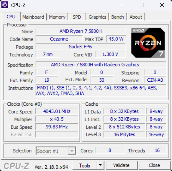
Locality of Reference
Programs tend to reuse the instructions and data they used recently. As a rule of thumb, 90% of the execution time of a program is spent in 10% of the code (the 90/10 rule), because of loops, procedures calling each other, and arrays accessed sequentially.
- Temporal locality: an item that is referenced tends to be referenced again soon (the instructions of a loop).
- Spatial locality: items near a referenced item tend to be referenced soon (consecutive instructions, elements of an array).
In pipelining we assume that memory operates at processor speed. The cache is the hardware that makes this possible: a small, fast memory that provides the memory objects referenced by the processor directly, most of the time.
Performance of a Memory Hierarchy
Consider two levels $M_1$ (e.g. cache) and $M_2$ (e.g. main memory), with cost per bit $c_i$ and capacity $S_i$.
$$\text{Average cost per bit } c = \frac{c_1 S_1 + c_2 S_2}{S_1 + S_2}$$For $c$ to approach $c_2$ we need $S_1 \ll S_2$.
The hit ratio $H$ is the probability that an address generated by the CPU refers to $M_1$. If $N_1$ and $N_2$ references go to $M_1$ and $M_2$, then $H = N_1/(N_1 + N_2)$; $1 - H$ is the miss ratio. With access times $t_{A1}$, $t_{A2}$ and miss penalty $t_{\text{miss}}$:
$$t_A = H\,t_{A1} + (1 - H)\,t_{\text{miss}}$$The miss penalty can be estimated in different ways:
- The word is accessed directly from $M_2$: $t_{\text{miss}} = t_{A2}$.
- The block containing the word is transferred to $M_1$ (time $t_B$), and the word is then accessed in $M_1$: $t_{\text{miss}} = t_B + t_{A1}$.
- Including the time $t_{\text{hit}}$ to check for a hit: $t_{\text{miss}} = t_{\text{hit}} + t_B + t_{A1}$.
Two cases of the word-access model are often named:
- Simultaneous (parallel) access: $M_1$ and $M_2$ are searched together, and a miss costs only $t_{A2}$: $$t_A = H\,t_{A1} + (1 - H)\,t_{A2}$$
- Hierarchical (sequential) access: $M_2$ is accessed only after $M_1$ misses, so a miss costs $t_{A1} + t_{A2}$: $$t_A = H\,t_{A1} + (1 - H)\,(t_{A1} + t_{A2}) = t_{A1} + (1 - H)\,t_{A2}$$
For example, with $H = 0.9$, $t_{A1} = 10$ ns and $t_{A2} = 100$ ns these give 19 ns and 20 ns.
With $r = t_{A2}/t_{A1}$ and $t_{\text{miss}} = t_{A2}$, the access efficiency and the speedup due to the hierarchy are
$$e = \frac{t_{A1}}{t_A} = \frac{1}{H + (1 - H)\,r}, \qquad S = \frac{t_{A2}}{t_A} = \frac{1}{H/r + (1 - H)}$$The speedup also follows from Amdahl’s law, with $F = H$ and speedup $r$.
The cache is 6 times faster than main memory and can be used 90% of the time. Find the speedup.
| Term | Meaning |
|---|---|
| Block (line) | smallest unit of information transferred between two levels |
| Hit rate | fraction of memory accesses found in the upper level |
| Hit time | time to access the upper level, including the time to determine hit or miss |
| Miss rate | fraction of memory accesses not found in the upper level |
| Miss penalty | time to replace a block in the upper level and transfer the missed block |
Level 1 has separate instruction and data caches. The clock cycle is 2 ns, the cache access time (including hit detection) is 1 cycle and the miss penalty is 15 cycles. 1% of instruction fetches and 8% of data references miss, and 20% of memory accesses are for data. Find the average access time.
A miss takes $1 + 15 = 16$ cycles. The average number of cycles per access is
$$0.8\,(0.99 \times 1 + 0.01 \times 16) + 0.2\,(0.92 \times 1 + 0.08 \times 16) = 0.92 + 0.44 = 1.36$$so $t_A = 1.36 \times 2 = 2.72$ ns.
For three levels (L1, L2 and main memory), a miss in L1 goes to L2:
$$t_A = H_{L1}\,t_{L1} + (1 - H_{L1})\,\big[H_{L2}\,t_{L2} + (1 - H_{L2})\,t_{\text{miss2}}\big]$$where $H_{L2}$ is the hit ratio of L2 for the accesses that reach it, and $t_{\text{miss2}}$ is the penalty when the data is in neither cache.
Cache Organization
The cache is divided into blocks (lines) of typically 8 to 256 bytes. When the CPU accesses a word, the hardware first checks whether it is in the cache. On a hit the word is read from the cache; on a miss the block containing the word is brought from main memory into the cache.
Fast Lookup
The lookup logic has to find an address $A$ among thousands of addresses in the cache directory, and the search must be fast.
- Linear search can take thousands of comparisons, and binary search tens.
- Hash search typically takes one comparison, independent of the number of entries. Hashing uses a table indexed by a hash function.
A simple hash function selects some bits of $A$:
The low-order bits select the byte within the block (the offset), the middle bits select the entry in the directory (the index), and the high-order bits are stored in the directory as the tag, which is compared to check that the entry holds the requested block.
A block serves the same purpose in cache memory as a page in virtual memory: it reduces the size of the translation table, and it exploits spatial locality. The cache directory has one entry for each block, as the page table has one entry for each virtual page. Main memory is also organized in blocks.
Four Questions of Cache Organization
- Block placement: where can a block be placed in the cache? (direct mapped, set associative)
- Block identification: how is a block found in the cache? (tag, valid bit, tag-checking hardware)
- Block replacement: which block is replaced on a miss? (LRU, FIFO, random)
- Write strategy: when is main memory updated on a write hit, and what happens on a write miss?
Block Placement
Direct Mapping
In a direct-mapped cache of $N$ blocks, memory block $M$ is placed in cache block $M \bmod N$.
A 32-bit address, a 16 KB cache and 32 B blocks. Find the widths of the tag, index and offset.
- Number of cache blocks $= 16\text{ KB}/32\text{ B} = 512$, so the index (which cache block) is $\log_2 512 = 9$ bits.
- The offset (which byte in the block) is $\log_2 32 = 5$ bits.
- The tag (which memory block is in this cache block) is $32 - 9 - 5 = 18$ bits.
The index is the low-order bits of the block number $M$ (that is, $M \bmod N$), and the tag is the remaining high-order bits. So consecutive memory blocks go to consecutive cache blocks, and two memory blocks compete for the same cache block only if they are a multiple of $N$ blocks (the cache size) apart, like blocks 6 and 14 above. The tag tells such blocks apart.
The problem with direct mapping: if a program alternately accesses $A, B, A, B, \dots$ and $A$ and $B$ map to the same cache block, every access is a miss, even if the rest of the cache is empty.
Set-Associative Mapping
In a set-associative cache the blocks are divided into $S$ sets. Memory block $M$ is placed in set $M \bmod S$, in any block of that set. If each set has $k$ blocks, the cache is $k$-way set associative.
The index field selects a set ($\log_2 S$ bits), and all the blocks in the set are checked in parallel:
- A direct-mapped cache is 1-way set associative ($S = N$).
- A fully associative cache has a single set ($S = 1$), so a block can be placed anywhere and there are no index bits. The tag is compared with all the tags in the cache, which needs a large associative memory (high cost, not scalable), but any replacement policy can be used.
- Typical values are 2, 4 or 8 ways. A set-associative cache needs several small associative memories, only one of which is used at a time.
| Mapping | Tag | Index / set | Word |
|---|---|---|---|
| Direct | 11 | 8 (256 blocks) | 5 |
| 4-way set associative | 13 | 6 (64 sets) | 5 |
| Fully associative | 19 | — | 5 |
In general, with block size $B$, $N$ cache blocks and $k$ ways:
$$\text{offset} = \log_2 B, \qquad \text{index} = \log_2 \frac{N}{k}, \qquad \text{tag} = \text{address bits} - \text{index} - \text{offset}$$Doubling the associativity moves one bit from the index to the tag. The tag directory has $N \times (\text{tag} + \text{valid} + \text{dirty} + \text{replacement bits})$ bits.
Block Identification
Each cache block has a tag. The tags of all the blocks where the requested block may be are compared with the tag field of the address, in parallel.
- Direct mapping: one comparison.
- $k$-way set associative: $k$ comparisons, in the selected set.
- Fully associative: a comparison with every tag.
A valid bit with each tag indicates whether the block contains valid data. If it is not set, the tag need not be matched.
Block Replacement
- With direct mapping there is no choice, since the placement is unique.
- With set-associative mapping, one block in the set must be selected:
- FIFO: the block that has been in the set longest;
- LRU: the block that has not been used for the longest time;
- Random: a randomly chosen block.
For LRU the hardware keeps track of usage in the cache directory; a 2-way cache needs 1 bit per set. In a 4-way cache, a 2-bit counter can be kept with each block:
- On a hit, the counter of the referenced block is set to 0, the counters lower than its original value are incremented, and the others are unchanged.
- On a miss, if the set is not full, the counter of the new block is set to 0 and all the others are incremented.
- On a miss, if the set is full, the block with counter 3 is replaced, its counter is set to 0, and the other three are incremented.
Write Policies
Reads dominate cache accesses: all instruction fetches are reads, and most instructions do not write to memory. A read can be done while the tag is compared, and the data is discarded on a miss. A write takes longer: only part of the block (1 to 8 bytes) is changed, so it is a read-modify-write, and it cannot begin until the tag check shows a hit.
Write Hit
Write through: the data is written both to the cache and to main memory.
- Cache and main memory are consistent; main memory has the latest data, which is needed for I/O and multiprocessors.
- A read miss does not cause a write to memory.
- Multiple writes to the same block cause high memory traffic, and a write has to wait for memory.
A write buffer is used to reduce the stall time: the CPU writes into the buffer, and the buffer writes to memory.
Write back: the data is written only to the cache. A modified block is written to memory only when it is replaced.
- A dirty (modified) bit is kept for each block; a clean block is not written back on replacement.
- Writes are done at cache speed, and several writes to a block need only one write to memory, so less memory bandwidth is used.
- The cache and memory copies are not always the same.
Write Miss
- Write allocate: the block is loaded into the cache, and the write is then done as a write hit.
- No-write allocate: the block is written directly in main memory and is not loaded into the cache.
The usual combinations are:
- write back with write allocate, so that later writes to the block are done in the cache;
- write through with no-write allocate, since later writes have to go to memory anyway.
| Cache | Operation | Penalty |
|---|---|---|
| Write through | write hit, no write buffer | $t_{MM}$ |
| Write through | write hit, perfect write buffer | 0 |
| Write back | write hit | 0 |
| Write back + write allocate | miss, replaced block clean | $t_{MM}$ |
| Write back + write allocate | miss, replaced block dirty | $2\,t_{MM}$ |
With a dirty replaced block, the old block is written to memory and then the new block is read, so the penalty is $2\,t_{MM}$.
Types of Cache Misses
- Compulsory miss (cold-start miss): the first access to a block is a miss, unless prefetching is used. It occurs even in an infinite cache. It can be reduced by a larger block size, which reduces the number of memory blocks.
- Capacity miss: a block is replaced because the cache cannot hold all the blocks the program needs, and is accessed again later. It would be avoided with a larger cache. To decide whether a miss is a capacity miss, the cache is assumed to be fully associative.
- Conflict miss: in a direct-mapped or set-associative cache, a block is replaced because several blocks map to the same set, and is accessed again later. It would not occur in a fully associative cache with LRU. Conflict misses increase from fully associative to set associative to direct mapped, and are reduced by higher associativity.
Physical memory is 1 MB and the cache is 8 KB, direct mapped, with 32 B blocks. Classify the misses for the block sequence 2, 216, 100, 256, 2048, 728, 256, 216.
The physical address is 20 bits: offset $\log_2 32 = 5$, index $\log_2 (8\text{ KB}/32\text{ B}) = 8$, and tag $20 - 8 - 5 = 7$ bits, since $1\text{ MB}/8\text{ KB} = 128$ memory blocks map to each cache block. Memory block $M$ goes to cache block $M \bmod 256$.
| Block | Cache block | Result |
|---|---|---|
| 2 | 2 | compulsory miss |
| 216 | 216 | compulsory miss |
| 100 | 100 | compulsory miss |
| 256 | 0 | compulsory miss |
| 2048 | 0 | compulsory miss (replaces 256) |
| 728 | 216 | compulsory miss (replaces 216) |
| 256 | 0 | conflict miss |
| 216 | 216 | conflict miss |
The first six are first accesses to their blocks. The last two blocks were in the cache and were replaced because of a conflict.
Cache and Programming
For the analysis, the program is viewed close to machine code, to see the loads and stores.
A data cache is 16 KB, direct mapped, write back, with 32 B blocks (tag 18, index 9, offset 5 bits). Find the hit ratio of the loop below, assuming i and sum are in registers and the cache is initially empty.
double A[2048], sum = 0.0;
for (i = 0; i < 2048; i++) sum = sum + A[i];
The reference sequence is load A[0], A[1], …, A[2047]. Let the base address of A be 0xA000. An element is 8 B, so 4 consecutive elements fit in a 32 B block.
| Element | Address | Result |
|---|---|---|
| A[0] | 0xA000 | miss (compulsory) |
| A[1]–A[3] | 0xA008–0xA018 | hit |
| A[4] | 0xA020 | miss (compulsory) |
| A[5]–A[7] | 0xA028–0xA038 | hit |
| ⋮ | ⋮ | ⋮ |
| A[2044] | 0xDFE0 | miss (compulsory) |
| A[2045]–A[2047] | 0xDFE8–0xDFF8 | hit |
Each block gives one compulsory miss and three hits, so the hit ratio is 75%.
Cache Performance
$$\text{effective } CPI = CPI_{\text{base}} + \text{memory stall cycles per instruction}$$The base CPI is 1.1, the instruction mix is ALU 50%, load 15%, store 15%, branch 20%, the miss rate is 1.5% and the miss penalty is 50 cycles. Find the effective CPI for a unified write-through, no-write-allocate L1 cache with (a) no write buffer, (b) a perfect write buffer, (c) a write buffer that eliminates 85% of the write stalls.
There are $1 + 0.15 + 0.15 = 1.3$ memory accesses per instruction: $1.15$ reads (instruction fetch and load) and $0.15$ writes.
- (a) All writes stall: $50 \times (1.15 \times 0.015 + 0.15) = 8.36$, so $CPI = 9.46$.
- (b) Only read misses stall: $50 \times 1.15 \times 0.015 = 0.86$, so $CPI = 1.96$.
- (c) $50 \times (1.15 \times 0.015 + 0.15 \times 0.15) = 1.99$, so $CPI = 3.09$.
For a write-back, write-allocate cache in which 10% of the blocks are dirty, a miss costs 50 cycles for a clean block and 100 for a dirty one:
$$\text{stalls per access} = 0.015\,(0.9 \times 50 + 0.1 \times 100) = 0.825, \qquad CPI = 1.1 + 1.3 \times 0.825 = 2.17$$Improving Cache Performance
$$\text{AMAT} = \text{hit time} + \text{miss rate} \times \text{miss penalty}$$The techniques reduce one of these three terms.
Reducing the miss rate:
- Larger block size. Reduces compulsory misses. But the miss penalty increases, and since there are fewer blocks, conflict and capacity misses may increase. High latency and high bandwidth of the lower level favour large blocks; low latency and low bandwidth favour small ones. Typical L1 block sizes are 32 to 64 bytes (64 B on the Ryzen 7 5800H).
- Larger cache. Reduces capacity misses, but increases the hit time, the cost and the power.
- Higher associativity. Reduces conflict misses, but increases the hit time and the power. As a rule of thumb, an 8-way cache is as effective as a fully associative one, and a direct-mapped cache of size $N$ has about the same miss rate as a 2-way cache of size $N/2$.
Reducing the miss penalty:
- Multi-level caches. The L1 cache is small enough to match the clock of the processor, and the L2 cache is large enough to capture many of the accesses that would go to main memory.
- The local miss rate of a cache is the number of its misses divided by the number of accesses to it: $\text{MissRate}_{L1}$, $\text{MissRate}_{L2}$.
- The global miss rate is the number of its misses divided by the total number of memory accesses by the processor: $\text{MissRate}_{L1}$ for L1, and $\text{MissRate}_{L1} \times \text{MissRate}_{L2}$ for L2.
- The local miss rate of L2 is large, since L1 takes most of the accesses, so the global miss rate is the more useful measure.
- Priority to read misses over writes. The write buffer may hold the updated value of a location needed on a read miss. Instead of waiting until the buffer is empty, the read miss checks the buffer for a conflict and continues if there is none.
Reducing the hit time:
- Avoiding address translation during cache indexing (next section).
In 1000 memory references there are 60 misses in L1 and 15 misses in L2. $\text{HitTime}_{L1} = 1$, $\text{HitTime}_{L2} = 12$ and $\text{MissPenalty}_{L2} = 180$ cycles. Find the miss rates and the AMAT (average memory access time).
$\text{MissRate}_{L1} = 60/1000 = 6\%$ (local and global). For L2, the local miss rate is $15/60 = 25\%$ and the global miss rate is $15/1000 = 1.5\%$.
$$\text{AMAT} = 1 + 0.06\,(12 + 0.25 \times 180) = 1 + 0.06 \times 57 = 4.42 \text{ cycles}$$- Multi-level inclusion: the data in L1 is always present in L2, so consistency between I/O and the caches can be checked in L2 alone.
- Multi-level exclusion: the data in L1 is never in L2; a miss in L1 swaps blocks between L1 and L2. This avoids wasting L2 space when L2 is only slightly larger than L1.
Note. In
SW $t1, 512($zero);LW $t2, 1024($zero);LW $t3, 512($zero), suppose 512 and 1024 map to the same block of a direct-mapped write-through cache, and the 4-word write buffer is not checked on a read miss. The stored value may still be in the write buffer when the last load misses and reads memory, so$t3may differ from$t1.
Other optimizations (Hennessy & Patterson):
- small and simple L1 caches, and way prediction, to reduce the hit time;
- pipelined and multi-banked caches, to increase the bandwidth;
- critical word first and early restart, to reduce the miss penalty;
- compiler optimizations, to reduce the miss rate;
- prefetching of instructions and data.
Caches and Address Translation
Two questions:
- Are real caches built on virtual or physical addresses?
- Do modern processors use pipelines of the kind studied here?
Every memory access needs a translation from virtual to physical address (by the memory management unit, MMU, and its translation lookaside buffer, TLB; see Part II), and the cache can be accessed before or after it.
Physically addressed cache (PIPT). The address is translated first, and the cache is indexed and tagged with the physical address. The hit time is higher, since every access goes through the MMU.
Virtually addressed cache (VIVT). The cache is indexed and tagged with the virtual address, and the MMU is used only on a miss. The problems are:
- Homonyms: the same virtual address in different processes refers to different data. Either the cache is flushed on a context switch, or the process id is included in each cache directory entry.
- Synonyms: different virtual addresses that translate to the same physical address can give more than one copy of a block in the cache.
- Page-level protection is not possible, and I/O (which uses physical addresses) complicates the design.
Virtually indexed, physically tagged cache (VIPT). The cache is indexed with virtual-address bits while the MMU translates, and the tag is compared with the physical address. This is typical of L1 caches. If the index and offset bits are all within the page offset, they are the same in the virtual and the physical address, and there are no synonyms:
$$\text{index bits} + \text{offset bits} \le \text{page-offset bits} \quad\Longleftrightarrow\quad \frac{\text{cache size}}{\text{associativity}} \le \text{page size}$$16 KB pages, 32-bit addresses, and a 64 KB direct-mapped cache with 32 B blocks.
- PIPT: the virtual page number (18 bits) is translated, and the physical address is split into tag 16, index 11 ($64\text{ KB}/32\text{ B} = 2048$ blocks) and offset 5 bits.
- VIPT: the page offset is $\log_2 16\text{K} = 14$ bits, but the index and offset need $11 + 5 = 16$ bits, so 2 index bits come from the virtual page number. Two virtual addresses for the same physical page that differ in these bits are placed in different sets (synonyms). A 4-way cache (16 KB per way) would avoid this.
Input/Output Organization
Secondary Storage
The organization of a magnetic disk (platters, tracks, sectors, cylinders), the disk access time and disk scheduling are covered in Part II. Typical values: 1 to 5 platters rotating at 5400 to 7200 rpm, 1000 to 5000 tracks per surface, 64 to 200 sectors per track, and sectors of 512 to 2048 bytes. The sector is the smallest unit that can be read or written. Modern disk units include a high-speed cache, and some use constant bit density, with more sectors on the outer tracks.
Note. One track passes under the head in one full rotation, not in the average rotational delay. At 7200 rpm a rotation takes 60/7200 s = 8.33 ms, so a track of 32 KB gives 32 KB / 8.33 ms ≈ 3,840 KB/s, and a track of 64 KB gives 64 KB / 8.33 ms ≈ 7.7 MB/s.
Solid-State Drives
A solid-state drive (SSD), or flash drive, is non-volatile, uses little power, is faster than a hard disk, and allows random access. Data is written in blocks (an erase followed by a write).
A flash cell is a floating-gate MOSFET (metal–oxide–semiconductor field-effect transistor): a MOS transistor whose gate is electrically isolated by an insulator, so the charge on it remains for a long time. The charge is controlled by the voltage on the control gate, and its presence or absence represents 0 or 1. To read a bit, a voltage $V_{\text{read}}$ is applied to the control gate and the drain current is measured: a programmed cell needs a higher control-gate voltage to conduct, so it gives (almost) no current.
| NOR | NAND | |
|---|---|---|
| Read | fast (~100 ns) | slower (~1 μs) |
| Write | slow (~10 μs) | fast (~1 μs) |
| Density | lower | higher (smaller cells) |
| Use | storing code (mostly read) | data storage |
In NAND flash, a page (e.g. 512 bytes) is read or written, and a block (a set of pages) is erased; a block must be erased before it is written. A cell can be erased or written about $10^6$ times, so wear leveling distributes the writes evenly over the whole array.
I/O Interface
Interfacing I/O devices is more complex than interfacing memory:
- There is a wide variety of peripherals (keyboard, mouse, disk, camera, printer, scanner).
- Their speeds vary widely, and the data transfer rate can be regular or irregular.
- The size of the data blocks transferred at a time varies widely, from a few bytes to kilobytes.
- They are slower than the processor and memory.
So a programmable I/O interface or I/O module is used. It interfaces to the processor and memory on one side, and to one or more I/O devices on the other.
In a typical device interface, the control logic operates the device according to the control signals from the I/O module and returns status signals to it, and a buffer holds the data being transferred [3].
Typical steps of an input operation:
- The processor asks the I/O module for the status of the device.
- The I/O module returns the status.
- If the device is ready, the processor requests the data transfer.
- The I/O module gets the data from the device.
- The I/O module transfers the data to the processor.
- The processor stores the data in memory.
Devices are connected through input and output ports:
- An output port is a PIPO (parallel-in parallel-out) register that is enabled when a particular output device address is given. Its inputs are connected to the data bus and its outputs to the device.
- An input port is a parallel tristate bus driver that is enabled when a particular input device address is given. Its outputs are connected to the data bus and its inputs to the device.
Memory-Mapped and I/O-Mapped Interfacing
Memory-mapped I/O: the same address decoder selects memory and I/O ports, and part of the memory address space is occupied by I/O devices. All the data transfer instructions for memory can be used for I/O. The processor needs no separate I/O instructions, and does not have to specify whether an address is a memory or an I/O address.
As an example, take a 16-bit address. A decoder on $A_{15} A_{14}$ selects three 16 KB memory modules with outputs 0 to 2, 48 KB in all. Output 3 enables a second decoder on $A_{13} A_{12}$, which selects ports A to D. The lower 12 bits are not decoded, so each port responds to a range of 4 K addresses.
I/O-mapped I/O: there are separate instructions for I/O data transfer (IN and OUT), and a processor signal identifies whether an address refers to a memory location or an I/O device. Separate address decoders select memory and I/O ports, and the complete memory address space can be used.
In the example below, $\text{IO}/\overline{\text{M}} = 0$ enables the memory decoder (for LD and SD), and $\text{IO}/\overline{\text{M}} = 1$ enables the I/O decoder through the inverter (for IN and OUT). All four 16 KB modules can now be used, 64 KB in all.
Data Transfer Techniques
- Programmed I/O: the CPU executes a program that transfers the data between the device and memory. It can be synchronous, asynchronous or interrupt-driven.
- Direct memory access (DMA): an external controller transfers the data directly between the device and memory, without CPU intervention.
Synchronous Transfer
The device transfers data at a fixed rate known to the CPU. The CPU initiates the I/O operation and transfers successive bytes or words after giving fixed time delays.
- The CPU lies idle during the delays.
- Not many devices have strictly synchronous characteristics.
- Errors may occur if the device and the processor get out of synchronization.
- A large number of words cannot be transferred in one go.
- The transfer speed depends not only on the speed of the device and memory, but also on the execution time of the code.
Asynchronous Transfer
The CPU does not know when the I/O module will be ready to transfer the next word, so it checks the status of the module to find out. This is called handshaking.
- While checking, the CPU cannot do anything else, which wastes CPU time for slow devices such as a keyboard or mouse.
- It is not suitable for high-speed devices with large blocks, since the CPU is tied up for the whole transfer.
- The transfer speed also depends on the execution time of the code.
An example is serial data transfer using start and stop bits. The devices are asynchronous at the level of bytes, but synchronous at the level of bits within a byte. The line is at 1 when idle. The receiver waits for a start bit (0), then reads the 8 data bits after known bit delays, least significant bit first, and the stop bit (1) separates the bytes [2].
Interrupt-Driven Transfer
The CPU initiates the transfer and proceeds to perform some other task. When the I/O module is ready, it informs the CPU by activating a signal called the interrupt request (INTR). The CPU suspends its task, services the request (carries out the transfer), and returns to the task. The part of the program that is activated by the request is the interrupt handler or interrupt service routine (ISR).
CPU time is not wasted in checking the status of the I/O module. It is needed only for the transfer itself, plus some overhead for transferring and returning control.
An ISR differs from a normal function:
- A function is called from well-defined places in the calling program, so only the relevant registers need to be saved on entry and restored before return.
- An ISR can be invoked from anywhere in the executing program, depending on when the request arrives. So potentially all the registers used in the ISR must be saved and restored.
Interrupt Handling
When an interrupt request arrives:
- At the end of the current instruction, the PC and the program status word (PSW), which holds the status flags and other processor status information, are saved on the stack automatically.
- The interrupt is acknowledged and the interrupt vector is obtained, based on which control transfers to the appropriate ISR. Different devices may have different ISRs.
- After handling the interrupt, the ISR executes a special return from interrupt (RTI) instruction, which restores the PSW and returns control to the saved PC. A normal RETURN does not restore the PSW.
An instruction cycle has several machine cycles, five in MIPS32. The interrupt is acknowledged only at the end of the last one.
The signals between the device controller and the CPU work as follows:
- The device controller sends INTR to the CPU.
- The CPU finishes the current instruction and sends back interrupt acknowledge (INTA).
- The device controller sends the interrupt vector (or number) over the data bus.
- The CPU reads the vector and identifies the device, and so the correct ISR.
The vector is put on the data bus through a tristate buffer enabled by INTA.
Priority Interrupt Controller
When several devices can interrupt the CPU, a common solution is a priority interrupt controller, which interacts with the CPU on one side and the devices on the other.
The INTR line to the CPU is active when any device activates its request line, $\text{INTR} = \text{INTR}_0 + \text{INTR}_1 + \dots + \text{INTR}_n$. When the CPU sends back INTA, the controller sends the corresponding acknowledge to the interrupting device and puts its vector on the data bus.
The controller is programmable: the vectors of the various interrupts can be specified. When more than one request is active at a time, a priority mechanism is used (e.g. $\text{INTR}_0$ is the highest, followed by $\text{INTR}_1$).
Interrupt Nesting
Suppose device D0 has interrupted and the CPU is executing its ISR, and in the meantime device D1 interrupts. There are two possibilities:
- D1 interrupts the ISR for D0 and gets processed first, and then the ISR for D0 is resumed. This creates a problem for multi-level nesting.
- The interrupt system is disabled automatically whenever an interrupt is acknowledged, so that handling of nested interrupts is not required.
Typical instruction sets have EI (enable interrupt) and DI (disable interrupt) instructions. In the second case the ISR executes EI just before RTI, and some ISAs combine the two into one instruction. DI is also used by the operating system to run code atomically, such as the semaphore wait and signal operations.
Cases That Make Interrupt Handling Difficult
For some interrupts, the current instruction cannot be finished. A special RETURN instruction is then needed, which returns and restarts the interrupted instruction. Examples are a page fault (the location being accessed is not in main memory) and an arithmetic exception (e.g. division by zero).
Handling Multiple Devices
With several devices capable of generating interrupts, four questions arise: how the CPU identifies the interrupting device, how it finds the starting address of the ISR, whether nesting is allowed, and how simultaneous requests are handled.
Device Identification
Suppose the devices share a common request line, $\text{INTR} = \text{INTR}_1 + \text{INTR}_2 + \dots + \text{INTR}_n$. Each device can have a status bit showing whether it has interrupted, and the CPU can poll the status bits to find out which one did.
A better alternative is the interrupt vector: the interrupting device sends a special identifying code on the data bus on receiving INTA.
Starting Address of the ISR
For a processor with several request inputs, the ISR address can be fixed for each input, but this lacks flexibility. With vectors, the device identifies itself and the CPU looks up the ISR address in a table. The interrupt latency is somewhat increased, since the CPU does not jump to the ISR immediately.
Nesting
A simple approach is to disable all interrupts during an ISR. ISRs are typically short, so the delay to a second request is often acceptable. Otherwise, some devices are given higher priorities (e.g. a timer that maintains a real-time clock), and a higher-priority interrupt may interrupt the ISR of a lower-priority one.
Simultaneous Requests
The CPU needs a mechanism by which only one request is serviced, while the others are delayed or ignored. If it has several request lines, it can use a priority scheme and accept the request with the highest priority.
With polling, priority is assigned automatically by the order in which the devices are polled.
Priority can also be set by daisy chaining: the INTR line is common to all devices, but INTA propagates serially through them. A device that receives INTA passes it on only if it has not interrupted. Otherwise it stops the propagation and puts its identifying code on the data bus. So the device electrically closest to the CPU has the highest priority.
Types of Interrupts
- Hardware interrupt: the signal comes from a device external to the CPU (keyboard, mouse, timer).
- Maskable: can be masked or delayed when a higher-priority request arrives. Processor instructions can selectively mask and unmask the request lines.
- Non-maskable: cannot be delayed and must be handled immediately (power failure).
- Software interrupt: caused by executing an instruction, not by external inputs.
- Trap: a special instruction that requests a service from the operating system, also called a system call.
- Exception: an unplanned interrupt generated from within the system while a program executes (invalid opcode, division by zero, page fault, invalid memory access).
Direct Memory Access
In programmed I/O, machine instructions transfer the data between the device and memory. This is not suitable for transferring large blocks at high speed, for two reasons [3]:
- The transfer rate is limited by how fast the processor can test and service the device. Several instructions, with their memory accesses, are executed for each word, since they also increment the memory address and keep track of the word count [2]. With 20 instructions per word at 1 GHz and CPI 1, a word takes 20 ns, i.e. at most 50 M words/s.
- The processor is tied up managing the transfer. With status checking it does nothing else until the transfer is over, and with an interrupt for each word, the overhead of the ISR is added to every word [2] [3].
A disk has a synchronous mode of operation: once the head reaches the track, the data arrives at a fixed rate. A 7200 rpm disk with 64 KB per track delivers 64 KB / 8.33 ms ≈ 7.7 MB/s, which for 32-bit words is one word every 520 ns. The 20 ns per word above can keep up with this, but with status checking the CPU is occupied for the whole block.
With direct memory access (DMA), a block is transferred directly between a device and memory without continuous CPU intervention.
DMA Controller
A hardwired DMA controller carries out the transfer, so no instructions are executed for it. The maximum speed is determined by the rate of the memory read and write operations, which is much faster than programmed I/O.
- The CPU initializes the DMA controller.
- When the device is ready, the DMA controller sends DMA-RQ to the CPU.
- At the next DMA breakpoint, the CPU releases the bus (puts its bus lines in the high-impedance state) and sends DMA-ACK.
- The DMA controller transfers the data directly to or from memory.
- When the transfer is done, it removes DMA-RQ, the CPU uses the bus again, and the DMA controller sends an interrupt to the CPU.
For every DMA channel, the controller has three registers, which the CPU initializes before each transfer: the memory address, the word count, and the address of the data on the disk.
A DMA request can be acknowledged at the end of any machine cycle, since the CPU only gives up the bus and its state is not changed. An interrupt is acknowledged only at the end of an instruction, since the ISR changes the processor state.
DMA Transfer Modes
- Cycle stealing: the DMA controller requests the bus for a few cycles (1 or 2), preferably when the CPU is not using memory, and returns it after each word. It is said to steal cycles from the CPU without the CPU knowing it.
- Block (burst) transfer: the DMA controller transfers the whole block without interruption. This gives the maximum possible data rate, but the CPU lies idle during the transfer, as it cannot fetch instructions from memory.
If the device takes time $X$ to prepare a block and the DMA takes time $Y$ to transfer it, the CPU is blocked for a fraction $Y/(X + Y)$ of the time in burst mode. With cycle stealing it is blocked only for the memory cycles actually stolen, i.e. (cycle time) / (time between words) per word.
Other Applications of DMA
Other than transfers to and from high-speed peripherals, DMA can be used for:
- High-speed memory-to-memory block moves.
- Refreshing dynamic memory, by periodically generating dummy read requests to the columns.
Exercises on I/O Transfer
The slides give these exercises without solutions. Data rates are taken with 1 KB = 1000 B.
2048 bytes are read in programmed I/O mode with a 32-bit bus. Each interrupt takes 4 μs to service (transferring 32 bits). How much CPU time is needed?
$2048/4 = 512$ interrupts, so $512 \times 4\ \mu\text{s} = 2048\ \mu\text{s} \approx 2.05$ ms.
A DMA module transfers bytes from a device at 76800 bit/s. The CPU fetches 2 million 32-bit instructions per second. How much is the processor slowed down?
The device delivers $76800/8 = 9600$ bytes/s, and each byte takes one memory cycle. The CPU uses $2 \times 10^6$ memory cycles per second for instruction fetches, so the slowdown is $9600/(2 \times 10^6) = 0.48\%$.
A DMA controller transfers 32-bit words to memory by cycle stealing. The words are assembled from a device that sends 2400 bytes/s. The CPU executes $10^6$ instructions per second. How much is the CPU slowed down?
$2400/4 = 600$ words/s, i.e. 600 stolen cycles per second, so the slowdown is $600/10^6 = 0.06\%$.
A device transfers 8 KB/s continuously with interrupt-driven I/O, interrupting for every byte. The interrupt processing takes 100 μs, and the ISR takes 8 μs to transfer the byte. What fraction of CPU time does the device take?
Each byte costs $100 + 8 = 108\ \mu$s, and there are 8000 bytes per second: $8000 \times 108\ \mu\text{s} = 0.864$ s per second, i.e. 86.4% of the CPU time.
A disk has 16 surfaces, 512 tracks per surface, 512 sectors per track, 1024 bytes per sector, and rotates at 3600 rpm. It uses cycle stealing, transferring one 4-byte word per DMA cycle, and the memory cycle time is 40 ns. Find the maximum percentage of time the CPU is blocked.
A track holds $512 \times 1024 = 2^{19}$ bytes and is read in one rotation, $1/60$ s, so the transfer rate is $2^{19} \times 60 \approx 31.46 \times 10^6$ bytes/s. A 4-byte word arrives every $4/(31.46 \times 10^6) \approx 127$ ns, and each word blocks the CPU for one 40 ns memory cycle: $40/127 \approx 31.5\%$.
A disk is connected through DMA to a 50 MHz processor. Setting up a DMA transfer takes 2000 cycles, and handling the completion interrupt takes 1000 cycles. The disk transfers 4000 KB/s in blocks of 8 KB on average, during idle CPU cycles. What fraction of the processor time does the disk use?
$4000/8 = 500$ blocks per second, each costing $2000 + 1000 = 3000$ cycles: $500 \times 3000 = 1.5 \times 10^6$ cycles out of $50 \times 10^6$, i.e. 3%.
A device of 20 KB/s transfers data byte by byte. The interrupt overhead is 6 μs, and the transfer time between the interface register and the CPU or memory is negligible. What is the minimum performance gain of interrupt-driven mode over programmed (busy-wait) mode?
With busy waiting, the CPU is occupied for the whole transfer. With interrupts, it is occupied for $20\,000 \times 6\ \mu\text{s} = 0.12$ s per second of transfer. So the gain is at least $1/0.12 \approx 8.3$.
Device Interfacing Examples
Keyboard. A keyboard is a set of push-button switches. With one key per port line, $N$ keys need $N$ lines; arranged as a matrix, they need $2\sqrt{N}$ lines.
- To detect a key press, all rows are set to 0 and the columns are read; if any column bit is 0, a key is pressed.
- To find which key (keyboard scanning), one row at a time is set to 0 and the columns are checked, giving the row and column of the key.
- For interrupt-driven operation, the rows are grounded through AND gates with a control input set to 0, and the column lines go to a NAND gate whose output is connected to INTR, so a key press raises an interrupt. In the ISR the control input is set to 1 and the keyboard is scanned.
Printer. Older printers used a serial port (RS-232C) or a parallel port (LPT, 25 pins, 8 data lines). With the parallel port, the CPU sends the data and activates STROBE; the printer activates BUSY while printing and sends ACK when done (asynchronous transfer with handshaking). Modern printers use USB.
Buses
A bus is a collection of wires through which data is transmitted: the data bus carries the data, and the address bus carries where it should go. The bus protocol is the set of rules for the format and transmission of data.
- Parallel bus: fast, but costly over long distances and subject to interference between lines at high frequency. Serial bus: cheap over long distances, without interference, but slower.
- The device that controls the bus is the master, the others are slaves.
- The system bus connects CPU and memory; the front-side bus connects the CPU to the north bridge; the back-side bus connects the CPU to the L2 cache; the memory bus connects the north bridge to memory; a graphics bus (AGP in older PCs, now PCI Express) connects the north bridge to the GPU (graphics processor); expansion buses (ISA and PCI in older PCs, now PCI Express) and USB connect to peripherals.
- Bus width is the number of data wires, and bus bandwidth the amount of data transferred per unit time (e.g. PCI 127 MB/s, PCI-Express 16× v2 8000 MB/s).
In a synchronous bus a common clock controls the operations. For a memory read, the CPU places the address, asserts MREQ and RD once the address is stable, the memory places the data, and the CPU reads it and removes MREQ and RD.
In an asynchronous bus there is no common clock, and the master and slave handshake:
- The CPU places the address, and asserts MREQ and RD when the address is stable.
- The CPU asserts MSYN, and the memory controller accesses the memory.
- The memory controller places the data on the data lines and asserts SSYN.
- The CPU takes the data and removes MREQ, RD and MSYN.
- The memory controller removes SSYN.
Bridge-based architectures separate the buses by bridges, so that different buses can operate in parallel.
Universal Serial Bus
USB connects almost all kinds of peripherals (keyboard, mouse, printer, disks, cameras, phones). It was developed from 1994 by seven companies to replace the variety of connectors and to simplify the software configuration of devices.
| Version | Year | Maximum rate |
|---|---|---|
| USB 1.1 | 1998 | 12 Mbit/s |
| USB 2.0 | 2000 | 480 Mbit/s |
| USB 3.0 | 2008 | 5 Gbit/s |
| USB 3.1 | 2013 | 10 Gbit/s |
Data is sent serially with differential NRZI (non-return-to-zero inverted) encoding: a 0 is sent as a change of signal level and a 1 as no change. Bit stuffing guarantees a minimum frequency of transitions: a 0 is inserted after every six consecutive 1s, e.g. 1101 1111 1101 0100 → 1101 1111 10101 0100.
USB uses a tiered star topology: all devices are connected to a root hub, through hubs, up to 127 devices. The cable has 4 wires (power, ground and two differential signal lines). USB is a polled bus: all transactions are initiated by the host.
- Host: controls the system (usually the computer) and contains the software drivers that schedule transactions and read the device configurations. Its physical interface to the root hub is the host controller.
- Hub: detects new devices and keeps their status, acts as a repeater for the signals, and isolates the devices electrically, so malfunctioning devices can be removed and slower devices put on a separate branch.
- Device: a slave that only responds to reads and writes and never initiates them. It contains registers with its configuration information.
The client software decides what data to transfer, the USB system software schedules when and how often, and the host controller composes and regulates the transfers. The Type-A plug goes into a host or hub, the Type-B plug into a device, with mini and micro versions for small devices. Type-C plugs can deliver up to 20 V at 5 A (100 W), and Thunderbolt 3 uses the same connector, at up to 40 Gbit/s.
Pipelining
Basic Concepts
Pipelining is the overlapped execution of several instructions (or input sets) by partitioning a computation into $k$ sub-computations, called stages.
The increase in hardware cost is small, and the ideal speedup is $k$. Pipelining is used in instruction execution, in arithmetic (the same operation on several data sets) and in memory access (consecutive locations).
With $k$ stages of one cycle each and $n$ instructions:
- Serial (non-pipelined): each instruction takes $k$ cycles, so $n$ instructions take $k \cdot n$ cycles.
- Pipelined: $k - 1$ cycles fill up the pipeline, and then one instruction completes every cycle (CPI = 1), so $n$ instructions take $n + k - 1$ cycles.
A speedup of $k$ could also be obtained by replicating the hardware $k$ times, but the cost would also be $k$ times. Splitting the computation into stages needs only latches between the stages, to hold the intermediate results.
Synchronous k-Stage Pipeline
Let $t_i$ be the delay of stage $S_i$ and $d_L$ the delay of a latch. The clock period is set by the slowest stage:
$$\tau = \tau_m + d_L, \qquad \tau_m = \max_i t_i, \qquad f = \frac{1}{\tau}$$The minimum clock period must satisfy
$$\tau \ge t_{\text{skew} + \text{jitter}} + t_{\text{logic} + \text{setup}}$$- Skew: the maximum delay difference between the arrival of the clock at different latches.
- Jitter: the maximum delay difference between the arrival of the clock at the same latch.
- Logic delay: the maximum delay of the slowest stage.
- Setup time: the minimum time a signal must be stable at the input of a latch before it can be captured.
For $N$ tasks, ignoring the latch overheads:
$$T_k = [k + (N - 1)]\,\tau, \qquad T_1 = N k \tau$$$$\text{speedup } S_k = \frac{N k}{k + N - 1}, \qquad \text{efficiency } E_k = \frac{S_k}{k} = \frac{N}{k + N - 1}, \qquad \text{throughput } H_k = \frac{N}{[k + N - 1]\,\tau}$$A 4-stage pipeline has stage delays 60, 50, 90 and 80 ns, and a latch delay of 10 ns. Find the speedup over a non-pipelined unit for 1000 tasks.
The clock period is $\tau = 90 + 10 = 100$ ns, and the non-pipelined unit takes $60 + 50 + 90 + 80 = 280$ ns per task.
$$\text{Speedup} = \frac{1000 \times 280}{(4 + 999) \times 100} = \frac{280\,000}{100\,300} \approx 2.79$$For large $N$ the speedup tends to $280/100 = 2.8$, not 4, because the stages are not balanced.
A non-pipelined processor X has a clock of 250 MHz and CPI 4. Processor Y has a 5-stage pipeline, but because of latch delay and clock skew its clock is 200 MHz. For a program of 5000 instructions, find the speedup of Y over X and the MIPS rate of each.
$T_X = 5000 \times 4 / 250\text{ MHz} = 80\ \mu$s and $T_Y = (5 + 4999)/200\text{ MHz} = 25.02\ \mu$s, so the speedup is $80/25.02 = 3.2$. The MIPS rates are $250/4 = 62.5$ for X and $5000/25.02\ \mu\text{s} \approx 200$ for Y.
Types of Pipelines
- Degree of overlap: serial (the next operation starts after the previous one finishes), overlapped, or pipelined (fine-grain overlap).
- Depth: a shallow pipeline has few stages, each more complex; a deep pipeline has many stages, each simpler.
- Structure: in a linear pipeline the stages are executed in sequence; in a non-linear pipeline a stage may be used more than once for a data set (feedforward and feedback connections).
- Scheduling: a static pipeline executes the same sequence of stages for all data, and if one stalls all later ones are delayed; a dynamic pipeline can be reconfigured to perform different functions at different times.
Reservation Tables
A reservation table represents the utilization pattern of the stages of a synchronous pipeline: time steps on the $x$-axis and stages on the $y$-axis. The number of columns is the evaluation time.
For a linear pipeline the table is a diagonal. For a non-linear pipeline with stages A, B, C and two functions X and Y:
| 1 | 2 | 3 | 4 | 5 | 6 | 7 | 8 | |
|---|---|---|---|---|---|---|---|---|
| A | X | X | X | |||||
| B | X | X | ||||||
| C | X | X | X |
| 1 | 2 | 3 | 4 | 5 | 6 | |
|---|---|---|---|---|---|---|
| A | Y | Y | ||||
| B | Y | |||||
| C | Y | Y | Y |
- Multiple X’s in a row: repeated use of the same stage in different cycles.
- Continuous X’s in a row: extended use of a stage over more than one cycle.
- Multiple X’s in a column: several stages used in parallel during a clock cycle.
Pipeline Scheduling
The number of time units between two initiations is the latency. If two initiations try to use the same stage at the same time, there is a collision, and the latencies that cause a collision are forbidden latencies: the distances between two marks in the same row.
- X: row A gives 5, 7 and 2, row B gives 2, row C gives 2 and 4. Forbidden latencies $\{2, 4, 5, 7\}$.
- Y: row A gives 4, row C gives 2 and 4. Forbidden latencies $\{2, 4\}$.
The collision vector is $C = (C_m \dots C_2 C_1)$, where $C_i = 1$ if latency $i$ is forbidden and $m$ is the largest forbidden latency. Here $C_X = (1011010)$ and $C_Y = (1010)$.
From the collision vector a state diagram is constructed. The initial state is the collision vector. A latency $p$ is permitted if $C_p = 0$, and the next state is obtained by shifting the present state $p$ bits to the right and ORing it with the initial collision vector. A latency greater than $m$ returns to the initial state.
- A latency cycle is a latency sequence that repeats. In a simple cycle each state appears only once. A greedy cycle is formed by taking the minimum permitted latency from each state.
- Y: simple cycles (3), (5), (1, 5), (3, 5); greedy cycles (3) and (1, 5).
- X: simple cycles (3), (6), (8), (1, 8), (3, 8), (6, 8); greedy cycles (3) and (1, 8).
The minimum average latency (MAL) is 3 for both X and Y.
Scheduling algorithm: the collision vector is loaded into a shift register $R$. If the LSB (least significant bit) of $R$ is 1, no operation is initiated and $R$ is shifted right by one. Otherwise an operation is initiated, $R$ is shifted right by one and ORed with the original collision vector. Inserting non-compute delay stages into the pipeline changes the reservation table and may give a smaller MAL.
Arithmetic Pipelines
- Pipelined ripple-carry adder: latches are placed between the full adders. If a latch is about as slow as a full adder, the clock period is $T \ge t_{FA} + t_L$, and after the pipeline is full one sum is produced every $T$. This suits vector operations such as
a[i] = b[i] + c[i]. - Floating-point addition: compare the exponents, align the mantissas, add the mantissas, normalize the result (and round, for IEEE 754). For example, $0.9504 \times 10^3 + 0.8200 \times 10^2$: align to $0.0820$, add to get $1.0324$, normalize to $0.10324 \times 10^4$.
- Floating-point multiplication: add the exponents, multiply the mantissas, normalize, round.
An adder and a multiplier can be combined into one multifunction pipeline, scheduled with reservation tables.
Instruction Pipelining in MIPS32
The Five-Stage Pipeline
Each of the five steps IF, ID, EX, MEM and WB becomes a pipeline stage, each stage finishes in one clock cycle, and a new instruction is started every cycle.
| Stage | Instruction | Micro-operations |
|---|---|---|
| IF | all | IF/ID.IR ← Mem[PC] IF/ID.NPC, PC ← (taken branch ? EX/MEM.ALUOut : PC + 4) |
| ID | all | ID/EX.A ← Reg[rs] ID/EX.B ← Reg[rt] ID/EX.Imm ← sign-extend(IR₁₅..₀) |
| EX | R–R ALU | EX/MEM.ALUOut ← A func B |
| R–Imm ALU | EX/MEM.ALUOut ← A func Imm | |
| load / store | EX/MEM.ALUOut ← A + Imm EX/MEM.B ← ID/EX.B | |
| branch | EX/MEM.ALUOut ← NPC + (Imm ≪ 2) EX/MEM.cond ← (A == 0) | |
| MEM | ALU | MEM/WB.ALUOut ← EX/MEM.ALUOut |
| load | MEM/WB.LMD ← Mem[ALUOut] | |
| store | Mem[ALUOut] ← B | |
| WB | R–R ALU | Reg[rd] ← MEM/WB.ALUOut |
| R–Imm ALU | Reg[rt] ← MEM/WB.ALUOut | |
| load | Reg[rt] ← MEM/WB.LMD |
Without pipelining, $n$ instructions take $5Tn$; with pipelining they take $(4 + n)(T + \Delta)$, where $\Delta$ is the latch delay. The ideal speedup is about 5.
Requirements of the pipeline:
- An instruction is fetched every cycle, and there can be two memory accesses in a cycle (IF of one instruction, MEM of another). So the peak memory bandwidth is 5 times that of the non-pipelined version, and separate instruction and data caches are used.
- ID needs 2 register reads and WB needs 1 register write in every cycle. The register file has two read ports, and in MIPS32 the write is done in the first half of the cycle and the reads in the second half.
- PC is incremented in IF every cycle (in the non-pipelined version it is updated in MEM).
The latches increase the execution time of an individual instruction, but the throughput increases.
A MIPS32 processor runs at 1 GHz. Without pipelining, ALU operations and branches take 4 cycles and memory operations 5 cycles, with frequencies 50%, 15% and 35%. In the pipelined version, clock skew and setup time increase the clock cycle by 0.25 ns. Find the speedup.
Non-pipelined: $1\text{ ns} \times (0.5 \times 4 + 0.15 \times 4 + 0.35 \times 5) = 4.35$ ns per instruction. Pipelined: one instruction every $1.25$ ns. Speedup $= 4.35/1.25 = 3.48$.
Pipeline Hazards
A hazard is a situation that prevents an instruction from executing in its designated clock cycle. There are three types:
- structural hazards, due to resource conflicts;
- data hazards, due to data dependences between instructions;
- control hazards, due to branches and other instructions that change the PC.
A hazard can be avoided with additional hardware, or by inserting stall cycles. When an instruction is stalled, all the instructions after it are also stalled; the instructions before it continue, and no new instruction is fetched during the stall.
$$\text{Speedup} = \frac{C_{\text{nopipe}}}{C_{\text{pipe}}} \times \frac{\text{ideal CPI} \times \text{pipeline depth}}{\text{ideal CPI} + \text{stall cycles per instruction}}$$With ideal CPI 1 and the same clock cycle time:
$$\text{Speedup} = \frac{\text{pipeline depth}}{1 + \text{stall cycles per instruction}}$$Structural Hazards
Structural hazards arise when the hardware cannot support all combinations of overlapped instructions. Examples:
- a single memory for instructions and data: one instruction is fetched while another reads or writes data;
- a register read in ID while another instruction writes a register in WB;
- a functional unit (such as a floating-point multiplier) that is not fully pipelined.
Data references are 35% of the instructions and the ideal CPI is 1.3. How much faster is the machine without the memory structural hazard?
Structural hazards are allowed in real machines to reduce cost, when they are infrequent. The memory hazard is frequent, so separate instruction and data caches are used at the first level.
Data Hazards
Data hazards arise from data dependences between instructions in the pipeline. In ADD R2,R5,R8 followed by SUB R9,R2,R6, ADD writes R2 in WB (cycle 5) but SUB reads R2 in ID (cycle 3). Inserting stalls until R2 is written wastes 3 cycles. Two methods are used together to reduce the stalls:
- Data forwarding (bypassing): the result is in a pipeline register (e.g. EX/MEM.ALUOut) as soon as it is computed. Additional paths with multiplexers forward it to the ALU input of the instruction that needs it; the control unit detects the dependence and selects the path.
- Splitting the register access: the register write is done in the first half of the cycle and the reads in the second half, which removes the hazard between an instruction and the third instruction after it.
In MIPS32, memory references are always kept in order, so there are no data hazards between memory references: SW R2,100(R5) followed by LW R10,100(R5) is executed correctly. Cache misses can still cause stalls.
A load followed by an instruction that uses the loaded value causes a hazard that forwarding cannot remove: the data is available only at the end of MEM, and the next instruction needs it at the start of EX. The hardware (a pipeline interlock) detects the hazard in ID and stalls the instruction for one cycle before it is issued, i.e. moved from ID to EX.
The compiler tries to avoid a load followed by an immediate use (instruction scheduling). The slot after a load is the load delay slot; if the compiler cannot fill it with an independent instruction, it inserts a NOP (no-operation instruction).
; x = a - b; y = c + d
LW  R1, a
LW  R2, b
SUB R8, R1, R2   ; stall
SW  R8, x
LW  R1, c
LW  R2, d
ADD R9, R1, R2   ; stall
SW  R9, y
; scheduled: no stalls
LW  R1, a
LW  R2, b
LW  R3, c
SUB R8, R1, R2
LW  R4, d
SW  R8, x
ADD R9, R3, R4
SW  R9, y
The scheduled code uses two more registers (R3, R4) and has no load interlocks.
Dependences and Types of Data Hazards
Dependences are a property of the program. Whether a dependence results in a hazard, and whether the hazard causes a stall, are properties of the pipeline. For instructions $i$ and $j$, with $i$ before $j$ in program order:
- Data dependence (true dependence): $j$ uses a result produced by $i$, directly or through a chain of instructions. A value is transmitted from $i$ to $j$, so the order must be preserved.
- Name dependence: $i$ and $j$ use the same register or memory location (a name), but no value is transmitted between them through it. Since there is no flow of data, these are also called false dependences.
- Antidependence: $j$ writes a name that $i$ reads. The order must be preserved so that $i$ reads the correct (old) value.
- Output dependence: $i$ and $j$ write the same name. The order must be preserved so that the final value is the one written by $j$.
- Control dependence: whether $j$ is executed depends on a branch.
A name dependence can be removed by changing the name (register or memory location) used by one of the instructions, so that they no longer conflict. For registers this is register renaming, done statically by the compiler or dynamically by the hardware. A true dependence cannot be removed by renaming.
The data hazards are named by the order that must be preserved:
| Hazard | Problem | Dependence | Removed by renaming |
|---|---|---|---|
| RAW (read after write) | $j$ reads a source before $i$ writes it | true | no |
| WAR (write after read) | $j$ writes a destination before $i$ reads it | anti (name) | yes |
| WAW (write after write) | $j$ writes an operand before $i$ writes it | output (name) | yes |
RAR (read after read) is not a hazard.
DIV.D  F0, F2, F4
ADD.D  F6, F0, F8      ; RAW on F0 with DIV.D
S.D    F6, 0(R1)       ; RAW on F6 with ADD.D
SUB.D  F8, F10, F14    ; WAR on F8 with ADD.D
MUL.D  F6, F10, F8     ; WAW on F6 with ADD.D, WAR on F6 with S.D,
                       ; RAW on F8 with SUB.D
If the destination of SUB.D is renamed to T and that of MUL.D to S (with their later uses), the WAR and WAW hazards are removed and only the RAW dependences remain.
In the MIPS32 integer pipeline only RAW hazards are possible. All reads are done early (in ID), all writes late (in WB), and instructions complete in order, so WAR and WAW cannot occur. Of the RAW hazards, only a load followed by an immediate use causes a stall. WAW hazards are possible in pipelines where writes can happen in more than one stage (such as the multicycle floating-point pipeline below), and WAR hazards when instructions are reordered.
Control Hazards
Control hazards are caused by branches. If the branch is taken, the PC changes to a value other than PC + 4, and in the basic pipeline the PC is not updated until the end of MEM. The next instruction can be fetched only after that, so 3 cycles are lost. With 30% branches and ideal CPI 1, $CPI = 0.7 \times 1 + 0.3 \times 4 = 1.9$.
In MIPS32 a branch only tests a register for zero or compares two registers. With additional logic the outcome is known by the end of ID, and a separate adder computes the target address, so the penalty is one cycle.
Static techniques for reducing the branch penalty:
- Stall: freeze the pipeline and insert one stall cycle.
- Predict not taken: continue as if the branch were not taken, without changing the machine state until the outcome is known. If the branch is taken, the fetched instruction is discarded and the fetch restarts from the target. The penalty is 0 for a not-taken branch and 1 for a taken one.
- Predict taken: fetch from the target as soon as it is known. In MIPS32 the outcome and the target are known at the same time (end of ID), so there is no advantage; it is useful when the target is known before the outcome.
- Delayed branch: the $n$ instructions after a branch (the branch delay slots; $n = 1$ in MIPS32) are always executed, whatever the outcome. The compiler fills the delay slots with useful instructions, from before the branch, from the target, or from the fall-through path. Since the PCs of the delay slots and the target are not sequential, $n + 1$ PCs must be saved on an interrupt.
Ideal CPI 1, 5 stages, 20% branches of which 75% are taken. Find the speedup for the four techniques, taking an average penalty of 0.5 for the delayed branch.
- Stall: $5/(1 + 0.2 \times 1) = 4.17$.
- Predict taken: $5/(1 + 0.2 \times 1) = 4.17$.
- Predict not taken: $5/(1 + 0.2 \times 0.75) = 4.35$.
- Delayed branch: $5/(1 + 0.2 \times 0.5) = 4.55$.
Dynamic Branch Prediction
- Branch prediction buffer (BPB): a small memory indexed by the lower bits of the branch address, holding a bit that says whether the branch was recently taken. The entry may belong to another branch with the same lower address bits. If the prediction is wrong, the bit is inverted. With a 1-bit scheme, a branch that is almost always taken is mispredicted twice when it is not taken. In an inner loop of 20 iterations, the branch is mispredicted on the last iteration and on the first iteration of the next execution, so it is predicted correctly 18 times out of 20 (90%), although it is taken 95% of the time.
- 2-bit prediction: the prediction changes only after two consecutive mispredictions.
The 2-bit scheme alone does not speed up the MIPS32 pipeline, since the outcome and the target are both known at the end of ID. To avoid the penalty, the next fetch address must be known by the end of IF, before the instruction is decoded.
The branch target buffer (BTB) stores the addresses of known branches and the predicted next PC for each. The PC of the instruction being fetched is compared with the addresses in the BTB. If it matches, the instruction is a branch predicted taken, and the predicted PC is used as the next PC; otherwise fetching proceeds normally.
| In BTB? | Prediction | Actual | Penalty (cycles) |
|---|---|---|---|
| yes | taken | taken | 0 |
| yes | taken | not taken | 2 |
| no | — | taken | 2 |
| no | — | not taken | 0 |
With 90% of the branches found in the BTB, 8% of the predictions incorrect and 75% of the branches taken, the branch penalty is $0.9 \times 0.08 \times 2 + 0.1 \times 0.75 \times 2 = 0.29$ cycles.
Conditional instructions remove some branches. if (X == 0) A = B; can be written as CMOVZ R2, R3, R1 instead of BNEZ R1, L; ADDU R2, R3, R0, which converts the control dependence into a data dependence.
Exceptions and Interrupts
Interrupts complicate the pipeline: several instructions are executing at once, and some interrupts (such as a page fault) force an instruction to be aborted before it completes and restarted later.
| Stage | Possible exceptions |
|---|---|
| IF | page fault, misaligned memory access, memory protection violation |
| ID | illegal opcode |
| EX | arithmetic exception |
| MEM | page fault, misaligned memory access, memory protection violation |
| WB | none |
When an interrupt occurs, the state is saved as follows: a TRAP instruction is forced into the pipeline at the next IF; all writes by the faulting instruction and the ones after it are disabled until the TRAP is taken; and the interrupt handler saves the PC of the faulting instruction. The RFE instruction reloads the PCs and restarts the interrupted instructions.
A pipeline has precise interrupts if it can be stopped so that the instructions before the faulting instruction complete, and the instructions after it can be restarted from scratch.
Precise interrupts are needed for page faults and IEEE arithmetic. Interrupts may occur out of order: a later instruction can cause an instruction page fault in IF (cycle 2) before an earlier one causes a data page fault in MEM (cycle 4). The hardware therefore records each interrupt in a status vector that is carried with the instruction, and checks it when the instruction reaches WB, so that interrupts are handled in order.
Multicycle Operations
Floating-point operations need more than one cycle in EX. Using a slower clock would slow down all other operations, so the EX stage is repeated, with several functional units:
- Latency: the number of cycles between an instruction that produces a result and an instruction that uses it.
- Initiation interval: the number of cycles that must elapse between issuing two operations of the same type.
| Functional unit | Latency | Initiation interval |
|---|---|---|
| Integer ALU | 0 | 1 |
| Data memory (integer / FP load) | 1 | 1 |
| FP add / subtract | 3 | 1 |
| FP multiply | 6 | 1 |
| FP divide (not pipelined) | 24 | 25 |
Up to 4 FP adds, 7 FP multiplies and 1 FP divide can be outstanding. As a result:
- structural hazards occur on the divider, and when several instructions reach MEM or WB in the same cycle (in the slides’ example,
MUL.D F4,SUB.D F6andL.D F6all try to write the FP registers in the same cycle); - RAW hazards cause longer stalls (an
ADD.Dusing the result ofMUL.Dwaits for M7); - instructions complete out of order;
- WAW hazards are possible: in that example,
SUB.D F6andL.D F6both write F6.
Instruction-Level Parallelism
Instruction-level parallelism (ILP) is the overlap of independent instructions of one program, so that several are in execution at the same time. Unrelated instructions can be overlapped; related instructions must be separated by the latency between them.
for (i = 1000; i > 0; i--) x[i] = x[i] + s; with the latencies above (load to FP ALU 1, FP ALU to store 2) and one cycle of branch delay.
Loop: L.D    F0, 0(R1)      ; x[i]
      ADD.D  F4, F0, F2     ; + s
      S.D    F4, 0(R1)
      ADDI   R1, R1, #-8
      BNE    R1, R2, Loop
- As written: 9 cycles per iteration (1 stall after the load, 2 after ADD.D, 1 for the branch).
- Scheduled:
ADDIis moved after the load and the store offset changed to8(R1), giving 7 cycles per iteration. - Unrolled 4 times, with different registers (F0/F4, F6/F8, F10/F12, F14/F16) and one
ADDIandBNE: 14 instructions and 13 stalls, 27 cycles, i.e. 6.8 cycles per element. - Unrolled and scheduled (four loads, four adds, four stores): no stalls, 14 cycles, 3.5 cycles per element.
Loop unrolling replicates the loop body to reduce the loop overhead per iteration and to expose more instructions for scheduling.
With more than one instruction issued per cycle, the CPI can be less than 1:
- Superscalar: the hardware issues a small number (2 to 4) of independent instructions per cycle and checks for conflicts; if the instructions are dependent, only the first is issued. Issuing one integer and one FP instruction together needs little extra hardware, since they use different registers and functional units. In this version the next 3 instructions cannot use the result of a load without stalling, and the branch delay is 3 cycles.
- VLIW (very long instruction word): an instruction word of hundreds of bits specifies several operations, each for a different functional unit, sharing one register file. The compiler identifies the operations that can run together. With two memory units, one FP unit and one integer/branch unit, the unrolled loop takes 8 cycles for 4 elements, i.e. 2 cycles per element.
Dynamic Scheduling
In a statically scheduled pipeline, instructions are issued and executed in program order. If an instruction stalls, no later instruction can proceed, even an independent one:
DIV.D  F0, F2, F4
ADD.D  F10, F0, F8     ; waits for DIV.D
SUB.D  F12, F8, F14    ; independent, but stalls behind ADD.D
In dynamic scheduling the hardware rearranges the order of execution to reduce stalls, while preserving the data flow and the exception behavior. The ID stage is split into two stages:
- Issue: decode the instruction and check for structural hazards. Instructions are issued in program order.
- Read operands: wait until there are no data hazards, then read the operands. Instructions can bypass each other here, so execution is out of order, and so is completion.
Out-of-order execution creates WAR and WAW hazards, which cannot occur in the in-order five-stage pipeline:
DIV.D  F0, F2, F4
ADD.D  F6, F0, F8      ; waits for F0
SUB.D  F8, F10, F14    ; WAR on F8 with ADD.D
MUL.D  F6, F10, F8     ; WAW on F6 with ADD.D
If SUB.D is executed before ADD.D reads F8, ADD.D gets the wrong value. If MUL.D finishes before ADD.D, F6 is left with the value of ADD.D.
Scoreboarding executes an instruction as soon as its operands are available, which avoids RAW hazards. WAR and WAW hazards are handled by stalling: an instruction is not issued if its destination is the destination of an active instruction (WAW), and a result is not written while an earlier instruction still has to read the old value (WAR). The scoreboard is a central table that records the status of every instruction, functional unit and register.
Tomasulo’s Algorithm
Tomasulo’s algorithm also waits for the operands to avoid RAW hazards, but it removes WAR and WAW hazards by register renaming in hardware. Renaming changes the destination registers so that an out-of-order write does not affect an instruction that needs an earlier value. With two temporary registers S and T, the sequence above becomes
DIV.D  F0, F2, F4
ADD.D  S, F0, F8
SUB.D  T, F10, F14
MUL.D  F6, F10, T
and later uses of F8 must refer to T. The compiler can do this inside a basic block. The hardware can do it across branches, and it can use more names than there are architectural registers.
In Tomasulo’s scheme the names are the reservation stations. A reservation station is a buffer in front of a functional unit. It holds an issued instruction and either the values of its operands, if they are available, or the names of the reservation stations that will produce them. All results are broadcast on the common data bus (CDB), and every reservation station and register waiting for that result loads it at the same time. Hazard detection is distributed among the reservation stations, and results go directly to the waiting units instead of through the registers.
| Field | Meaning |
|---|---|
| Op | operation to perform on the source operands |
| Qj, Qk | reservation stations that will produce the source operands (0: operand available) |
| Vj, Vk | values of the source operands; for each operand only V or Q is valid |
| A | immediate field, then the effective address, of a load or store |
| Busy | the reservation station and its functional unit are occupied |
| Qi (register) | reservation station whose result is to be stored in the register (0: no pending write) |
An instruction goes through three steps, each of which can take any number of cycles:
- Issue: take the next instruction from the instruction queue (FIFO). If a reservation station of the right type is free, issue the instruction to it, with the operand values if they are in the registers, or else the names of the stations that will produce them. If no station is free, there is a structural hazard and the instruction stalls. This step renames the registers.
- Execute: if an operand is not available, monitor the CDB for it. When both operands are available, execute the operation. Waiting for the operands avoids RAW hazards. A load or store first computes its effective address, and loads and stores are kept in program order through this step.
- Write result: put the result on the CDB, from where it goes into the registers, the reservation stations and the store buffers waiting for it.
Show the reservation stations and register status for the following code when only the first load has completed and written its result (Hennessy & Patterson).
1. L.D    F6, 32(R2)
2. L.D    F2, 44(R3)
3. MUL.D  F0, F2, F4
4. SUB.D  F8, F2, F6
5. DIV.D  F10, F0, F6
6. ADD.D  F6, F8, F2
| Name | Busy | Op | Vj | Vk | Qj | Qk | A |
|---|---|---|---|---|---|---|---|
| Load1 | no | ||||||
| Load2 | yes | Load | 44 + Regs[R3] | ||||
| Add1 | yes | SUB | Mem[32 + Regs[R2]] | Load2 | |||
| Add2 | yes | ADD | Add1 | Load2 | |||
| Add3 | no | ||||||
| Mult1 | yes | MUL | Regs[F4] | Load2 | |||
| Mult2 | yes | DIV | Mem[32 + Regs[R2]] | Mult1 |
| Register | F0 | F2 | F4 | F6 | F8 | F10 |
|---|---|---|---|---|---|---|
| Qi | Mult1 | Load2 | Add2 | Add1 | Mult2 |
DIV.D already holds the value of F6 from the first load in Vk, so ADD.D, which writes F6, can complete before DIV.D starts without a WAR hazard. F6 is renamed to Add2: only the last instruction that writes a register updates it.
| Scoreboarding | Tomasulo | |
|---|---|---|
| RAW | wait for the operands | wait for the operands on the CDB |
| WAR | stall the write | renaming |
| WAW | stall the issue | renaming |
| Results passed through | registers | CDB |
| Hazard detection | central (the scoreboard) | distributed (reservation stations) |
Hardware Speculation
Branches limit dynamic scheduling, since an instruction after a branch cannot execute until the branch is resolved. With hardware speculation the processor predicts the branch and executes the instructions on the predicted path as if the prediction were correct. The results must not change the registers or memory until the prediction is known to be correct.
Tomasulo’s algorithm is extended with a reorder buffer (ROB), a FIFO queue that holds the results of instructions that have completed but not yet committed. Each entry has the instruction type (branch, store or register operation), the destination (register number or memory address), the value, and a ready bit. The ROB entries replace the reservation stations as the names used for renaming, and the ROB supplies operands to later instructions, as the reservation stations did.
The steps become:
- Issue: an instruction is issued if there is a free reservation station and a free ROB entry. The number of its ROB entry is the tag of its result.
- Execute: as before.
- Write result: put the result, tagged with the ROB entry, on the CDB, into the ROB and the waiting reservation stations.
- Commit: when the instruction at the head of the ROB has its result, write the result to the register (or memory for a store) and remove the entry. If the instruction is a mispredicted branch, the ROB is flushed and execution restarts at the correct successor.
Instructions execute out of order but commit in order. An exception is recorded in the ROB and raised only when the instruction reaches the head, so exceptions are precise, and an exception on a wrong path is never raised.
Modern processors issue several instructions per cycle with this scheme (a dynamically scheduled superscalar processor, e.g. the AMD Ryzen 7 5800H). Instead of keeping values in the ROB, they usually rename the architectural registers into a larger set of physical registers.
Parallel Architectures
Vector Processors
The performance gained from pipelining is limited by the clock cycle time (more stages give more dependences and a higher CPI) and by the instruction fetch and decode rate (the Flynn bottleneck). A vector processor has instructions that operate on entire arrays (vectors); one vector instruction is equivalent to a loop, with no loop overhead. For example, ADDV V1, V2, V3 adds two vectors of 64 elements.
- It consists of a pipelined scalar unit and a vector unit: vector registers (e.g. 8 registers of 64 double-words, each with 2 read ports and 1 write port), deeply pipelined vector functional units, and a pipelined load/store unit with interleaved memory.
- Deep pipelining causes no hazards between the elements, since each element is computed independently.
DAXPY (double-precision $a$ times $X$ plus $Y$): $Y = aX + Y$ for vectors of 64 elements.
The MIPS32 loop executes 514 instructions; the vector code has 6 (L.D, LV, MULTSV, LV, ADDVV, SV). Pipeline interlocks occur once per vector operation instead of once per element, about 64 times less often.
The time for a vector operation of length $n$ is
$$\text{start-up time} + n \times \text{initiation rate}$$The start-up time is determined by the pipeline depth, and the initiation rate is usually one result per cycle. A multiply with a start-up time of 12 cycles on 64 elements takes $(12 + 64)/64 = 1.19$ cycles per result. Independent vector operations on different units overlap: MULTV (start-up 7) and ADDV (start-up 6, starting one cycle later) both complete at cycle 71, i.e. 128 results in 71 cycles, or 1.8 FLOPS per cycle.
Other concepts: the vector length register specifies the length of a vector operation; strides allow vector elements that are not adjacent in memory; strip mining splits a loop over a long vector into loops over the hardware vector length.
Convoys and Chaining
A convoy is a set of vector instructions that can execute together: they have no structural hazards between them. With chaining, a dependent instruction can also be in the same convoy: the elements of the result of one vector unit are forwarded to the next unit as they are produced, as forwarding does for scalar results. A chime is the time to execute one convoy. A sequence of $m$ convoys on vectors of length $n$ takes about $m \times n$ cycles, ignoring the start-up time.
DAXPY with one load/store unit and chaining.
LV      V1, Rx          ; convoy 1: LV, MULTSV (chained)
MULTSV  V2, F0, V1
LV      V3, Ry          ; convoy 2: LV, ADDVV (chained)
ADDVV   V4, V2, V3
SV      V4, Ry          ; convoy 3: SV
There are 3 convoys, so 3 chimes: about $3 \times 64 = 192$ cycles, or 3 cycles per element. The two loads are in different convoys because there is only one load/store unit.
Multiple Lanes
A vector unit can have several lanes. Each lane has a part of the vector register file and one pipeline of each functional unit. With $m$ lanes, element $i$ of every vector register is in lane $i \bmod m$, so the lanes operate on different elements in parallel without communicating. With 4 lanes, one vector instruction completes 4 elements per cycle and a chime is reduced from 64 to 16 cycles.
Vector Mask Registers
A loop with an if cannot be vectorized directly:
for (i = 0; i < 64; i++)
    if (X[i] != 0)
        X[i] = X[i] - Y[i];
A vector mask register holds one bit per element. A compare instruction sets the mask, and the following vector instructions operate only on the elements whose mask bit is 1:
LV        V1, Rx        ; load X
LV        V2, Ry        ; load Y
L.D       F0, #0        ; F0 = 0
SNEVS.D   V1, F0        ; VM(i) = 1 if V1(i) != F0
SUBVV.D   V1, V1, V2    ; subtract under the mask
SV        V1, Rx        ; store X
The elements with mask bit 0 still take time in the pipeline, so the efficiency drops as fewer bits are 1.
Memory Banks
The memory system must supply one word per lane per cycle, while a memory bank needs several cycles (the bank busy time) before it can be accessed again. So the memory has many independent banks, interleaved by word address (memory interleaving, as in Memory Organization). With $b$ banks and stride $s$, an access returns to the same bank after $\text{LCM}(s, b)/s$ accesses, and there is a stall if this is less than the bank busy time.
8 banks, bank busy time 6 cycles, memory latency 12 cycles. Time to load a vector of 64 elements with stride 1 and with stride 32 (Hennessy & Patterson)?
- Stride 1: consecutive elements are in different banks, and a bank is used again only after 8 accesses, more than 6. Time $= 12 + 64 = 76$ cycles, 1.2 cycles per element.
- Stride 32: $32 \bmod 8 = 0$, so every element is in the same bank, and each access after the first waits for the bank busy time. Time $= 12 + 1 + 6 \times 63 = 391$ cycles, 6.1 cycles per element.
Gather and Scatter
Sparse matrices are accessed through index vectors. A gather (LVI, load vector indexed) loads the elements at base address + index vector; a scatter (SVI) stores them back the same way.
for (i = 0; i < n; i++)
    A[K[i]] = A[K[i]] + C[M[i]];
LV      Vk, Rk          ; load K
LVI     Va, (Ra+Vk)     ; gather A[K[i]]
LV      Vm, Rm          ; load M
LVI     Vc, (Rc+Vm)     ; gather C[M[i]]
ADDVV.D Va, Va, Vc
SVI     (Ra+Vk), Va     ; scatter A[K[i]]
The elements are in different banks in no particular order, so gathers and scatters are much slower than accesses with a fixed stride.
SIMD Instruction Set Extensions
Most general-purpose processors have SIMD (single instruction, multiple data) extensions: instructions that operate on several narrow elements packed in a wide register, e.g. eight 8-bit or four 16-bit operands in a 64-bit register. They were added for multimedia, where data is often 8 or 16 bits wide.
| Extension | Year | Register width |
|---|---|---|
| MMX | 1996 | 64 bits |
| SSE | 1999 | 128 bits |
| AVX | 2010 | 256 bits |
Compared with vector architectures, the SIMD extensions fix the number of elements in the opcode (no vector length register), and the early versions had no strided or gather/scatter accesses and no mask registers. Each increase in width added hundreds of new instructions, and AVX includes preparations to extend the width to 512 and 1024 bits [4]. They are easy to add to a processor, need little extra state for context switches, and need little memory bandwidth.
The Roofline Model
The arithmetic intensity of a program is the number of floating-point operations (FLOP) per byte of memory (DRAM) accessed. The roofline model bounds the performance of a program on a processor by its arithmetic intensity:
$$\text{Attainable GFLOP/s} = \min(\text{peak memory bandwidth} \times \text{arithmetic intensity},\ \text{peak floating-point performance})$$On a log–log plot this is a sloped line (memory-bound) joined to a horizontal line (compute-bound). The ridge point, where they meet, is the minimum arithmetic intensity needed to reach the peak floating-point performance.
Each Zen 3 core has two 256-bit FMA (fused multiply–add, $a \times b + c$ in one instruction) units (16 double-precision FLOP per cycle), so 8 cores at 3.2 GHz peak at $8 \times 3.2 \times 16 = 409.6$ GFLOP/s; two 64-bit DDR4-3200 channels give $2 \times 8 \times 3.2 = 51.2$ GB/s. The ridge point is at $409.6 / 51.2 = 8$ FLOP/byte. A kernel with an arithmetic intensity of 0.25 hits the slanted roof and is limited by memory bandwidth to $51.2 \times 0.25 = 12.8$ GFLOP/s; a kernel with an intensity of 16 hits the flat roof and runs at the peak 409.6 GFLOP/s. Measured (Stream) bandwidth is lower than the theoretical peak, which moves the ridge point to the right.
If the ridge point is far to the right, only kernels with a very high arithmetic intensity can reach the peak performance; if it is far to the left, almost any kernel can. Some kernels have an intensity independent of the problem size, $O(1)$ (sparse matrix–vector multiply, structured grids); others grow with it, $O(\log N)$ for FFTs (fast Fourier transforms) and $O(N)$ for dense matrix–matrix multiplication [4].
Hardware Multithreading
Instruction-level parallelism (ILP, see above) within one thread is limited, and long stalls such as cache misses leave the functional units idle. Multithreading lets several threads share the functional units of one processor. The processor keeps a separate state for each thread (register file, PC, page table register), and switches between threads much faster than an OS context switch.
- Fine-grained multithreading switches between threads every clock cycle, in round-robin order, skipping stalled threads. Short and long stalls of one thread are hidden by the others, but a thread that is ready to run is delayed by the others. Example: GPUs.
- Coarse-grained multithreading switches only on costly stalls such as L2 or L3 misses. A single thread runs at nearly full speed, but short stalls are not hidden, and the pipeline must be refilled after each switch.
- Simultaneous multithreading (SMT) issues instructions from several threads in the same cycle, on a dynamically scheduled multiple-issue processor. Register renaming keeps the registers of the threads apart, and the issue slots one thread leaves empty are filled by the others. Example: the AMD Ryzen 7 5800H runs two threads per core (8 cores, 16 threads).
Multicore Processors
A multicore processor has two or more independent cores on one die or package. Typically the L1 and L2 caches are private to each core and the L3 cache is shared. It is difficult to sustain Moore’s law and at the same time meet the performance demands of applications, mainly because the clock frequency is hard to increase without raising power consumption. So the hardware is replicated and run at a lower clock: two cores at 1.5 GHz can match one core at 3 GHz, with lower power, but only for work that can be split between them: by Amdahl’s law, the speedup from $N$ processors is $1/((1 - f) + f/N)$, where $f$ is the fraction of the execution time that can run in parallel [3]. In a symmetric multicore all the cores are identical; in an asymmetric one they may have different functions.
Note. Moore’s law: in 1965 Gordon Moore observed that the number of transistors per square inch on integrated circuits was doubling every year. The pace slowed to a doubling every 18 months in the 1970s, and has kept that rate since [3].
| Class | Meaning | Examples |
|---|---|---|
| SISD | single instruction stream, single data stream | uniprocessor |
| SIMD | single instruction stream, multiple data streams | vector and array processors, GPUs |
| MISD | multiple instruction streams, single data stream | no commercial machine |
| MIMD | multiple instruction streams, multiple data streams | multiprocessors |
- Tightly coupled multiprocessors: the processors share memory and communicate through it. The memory access time is the same for all processors (UMA, uniform memory access). Multicores are of this type. They are difficult to extend to many processors, since the memory bandwidth requirement grows with the number of processors.
- Loosely coupled multiprocessors: memory is distributed among the processors, which communicate through an interconnection network. Memory bandwidth scales, but the access time depends on the location of the data (NUMA), and communication is more complex and has higher latency.
Cache Coherence
If the same block is in the caches of two processors and one processor updates it, the data in the other cache and in memory become inconsistent. Cache coherence protocols are of two types:
- Snooping protocols: every cache monitors a shared bus. With write-invalidate, a processor that writes a block sends an invalidate, and the other copies are marked invalid.
- Directory-based protocols: a directory records which caches hold each block, and messages are sent only to those caches. This scales to more processors than a bus.
A snooping protocol can handle writes in two ways:
- Write invalidate: before writing, a processor gets exclusive access to the block by invalidating all other copies. A later read by another processor misses and gets the new value. This is used in almost all multiprocessors.
- Write update (write broadcast): every write is broadcast and all copies are updated. This uses much more bus bandwidth, since repeated writes to a block are all sent on the bus.
The MSI Protocol
In the MSI write-invalidate protocol with write-back caches, each cache block is in one of three states:
- Modified (M): the block has been written; this cache has the only valid copy, and memory is out of date.
- Shared (S): the block is clean and may be in other caches.
- Invalid (I): the block holds no valid data.
Each cache controller acts on requests from its own processor (read and write hits and misses) and on requests it snoops from the bus (read misses, write misses and invalidates for the block from other processors).
| State | Event | Action | Next state |
|---|---|---|---|
| Invalid | CPU read | place read miss on bus | Shared |
| Invalid | CPU write | place write miss on bus | Modified |
| Shared | CPU read hit | — | Shared |
| Shared | CPU write hit | place invalidate on bus | Modified |
| Shared | bus write miss or invalidate | — | Invalid |
| Modified | CPU read or write hit | — | Modified |
| Modified | bus read miss | write back the block | Shared |
| Modified | bus write miss | write back the block | Invalid |
A miss that replaces a block is handled the same way: a Modified block is written back first. When a Modified block is written back in response to a bus request, the memory access of the requesting processor is aborted and it gets the block from the write-back.
Two common extensions:
- MESI adds the Exclusive (E) state: the block is clean and in only this cache. A write to an Exclusive block needs no invalidate on the bus, which helps when a processor reads and then writes data no other processor uses.
- MOESI adds the Owned (O) state: the block is out of date in memory but may be shared; the owner supplies it on a miss and writes it back when it is replaced, so a read miss to a Modified block does not need a write to memory. AMD processors use MOESI.
Hazards Across Cores
The pipeline hazards are between instructions of one instruction stream, and the hardware detects them. Between processors, the ordering of accesses to shared data is the job of synchronization and of the memory consistency model.
Coherence and consistency are complementary: coherence defines the behaviour of reads and writes to the same memory location, while consistency defines the behaviour of reads and writes with respect to accesses to other memory locations [4].
A program is synchronized if every write of a variable by one processor and every access of that variable by another processor are separated by a pair of synchronization operations (for example an unlock after the write and a lock before the access). Accesses that are not ordered this way are data races: the outcome depends on the relative speed of the processors [4].
Sequential consistency requires that the result of any execution be the same as if the memory accesses of each processor were kept in order and the accesses of different processors were arbitrarily interleaved. Relaxed consistency models let reads and writes complete out of order, and use synchronization operations to enforce ordering, so that a synchronized program behaves as if the processor were sequentially consistent. Relaxing W→R gives total store ordering (processor consistency), relaxing W→W gives partial store order, and relaxing R→W and R→R gives weak ordering and release consistency [4].
Communication between processors also causes a fourth type of cache miss, the coherence miss (Hennessy & Patterson):
- True sharing miss: a processor reads a word that another processor wrote. The data is actually communicated. Such a miss would occur even with a block size of one word.
- False sharing miss: the block is invalidated because a word in it other than the one being read is written. The block is shared, but no word in it is actually shared, and the miss would not occur with a block size of one word.
Words x1 and x2 are in the same block, which is in the shared state in the caches of P₁ and P₂. Classify each access as a true sharing miss, a false sharing miss or a hit (Hennessy & Patterson).
| Time | P₁ | P₂ | Miss | Reason |
|---|---|---|---|---|
| 1 | write x1 | true sharing | x1 was read by P₂; its copy is invalidated | |
| 2 | read x2 | false sharing | block invalidated by the write of x1 | |
| 3 | write x1 | false sharing | block shared only because P₂ read x2 | |
| 4 | write x2 | false sharing | same as 3 | |
| 5 | read x2 | true sharing | x2 was written by P₂ |
False sharing is avoided by placing data used by different processors in different blocks (padding and alignment).
References
Sengupta, Indranil, and Kamalika Datta. Computer Architecture and Organization. NPTEL course, IIT Kharagpur. https://nptel.ac.in/courses/106105163.
Hamacher, Carl, Zvonko Vranesic, Safwat Zaky, and Naraig Manjikian. Computer Organization and Embedded Systems, 6th ed. McGraw-Hill, 2012.
Stallings, William. Computer Organization and Architecture: Designing for Performance, 10th ed. Pearson, 2016.
Hennessy, John L., and David A. Patterson. Computer Architecture: A Quantitative Approach, 5th ed. Morgan Kaufmann, 2012.