Introduction to Rendering
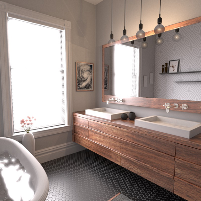
The goal of photorealistic rendering is to create an image of $3D$ scene that is indistinguishable from photograph of same scene. For the most part, we will be satisfied with an accurate simulation of the physics of light and its interaction with matter, relying on our understanding of display technology to present the best possible image to the viewer.
We mostly work with equations that model light as particles that travel along rays. This leads to a more efficient computational approach based on a key operation known as ray tracing
We are going to look at the Path Tracing algorithm. What are differences between Ray Tracing and Path Tracing? I got the following online:
I found a decent explaination in Unity forums here but I think of Ray Tracing as a general framework and Path Tracing a specialized way to do Ray Tracing.
Assumptions
- Light Travels in Straight Lines (in a uniform medium
- Lambert’s Cosine Law (Incident angle $\theta$ dictates surface illumination)
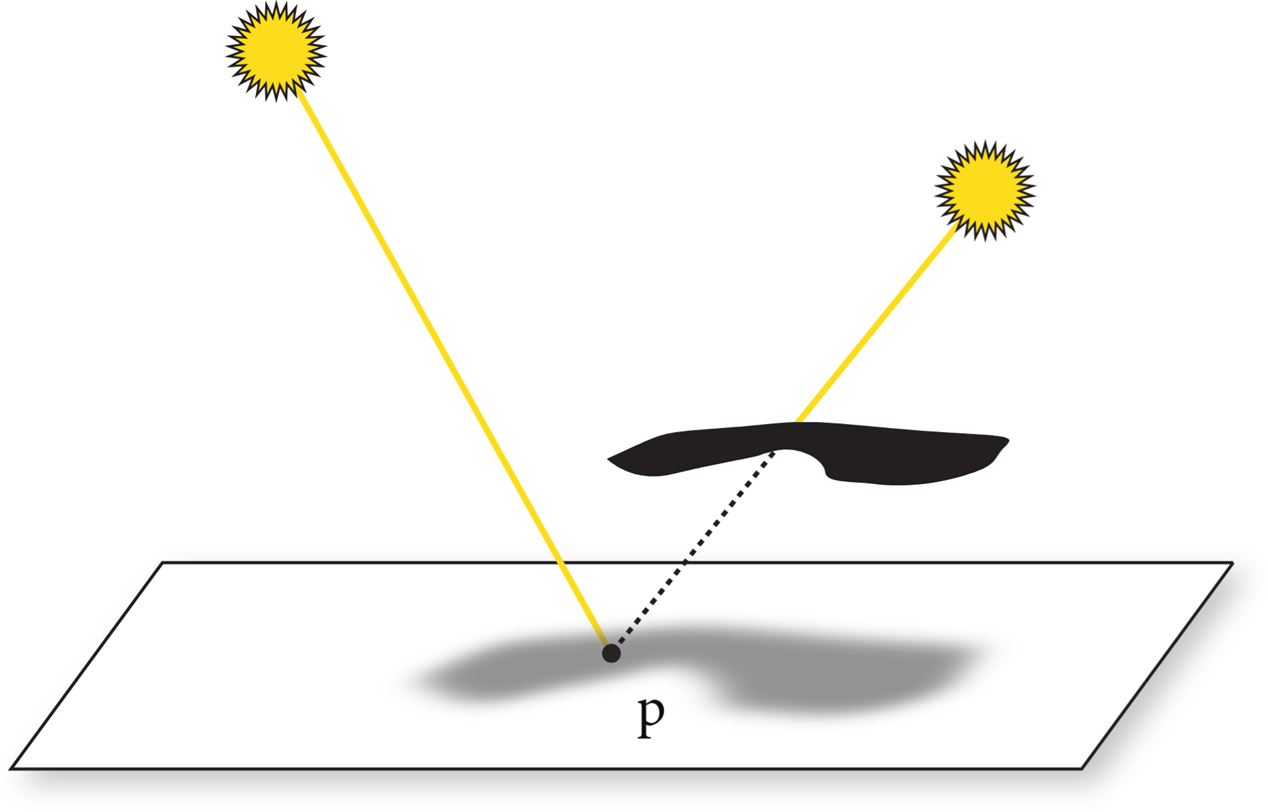
- Light is additive Size of light source affects shadow softness
- Inverse Square Law Intensidy decreases with distance form the souce $$Intensity \propto \frac{1}{r^2}$$
Components
Although there are many ways to write a ray tracer, all such systems simulate at least the following objects and phenomena:
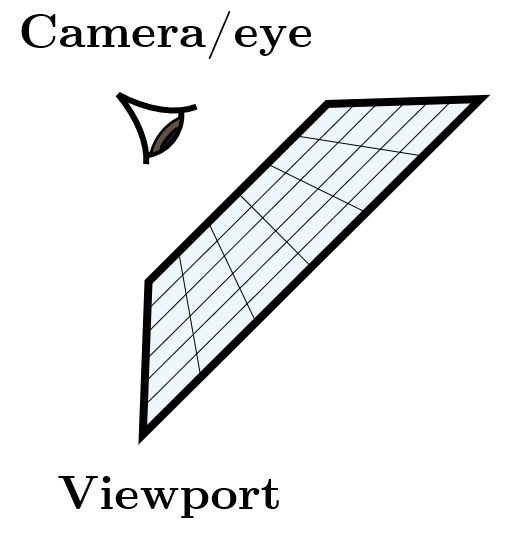
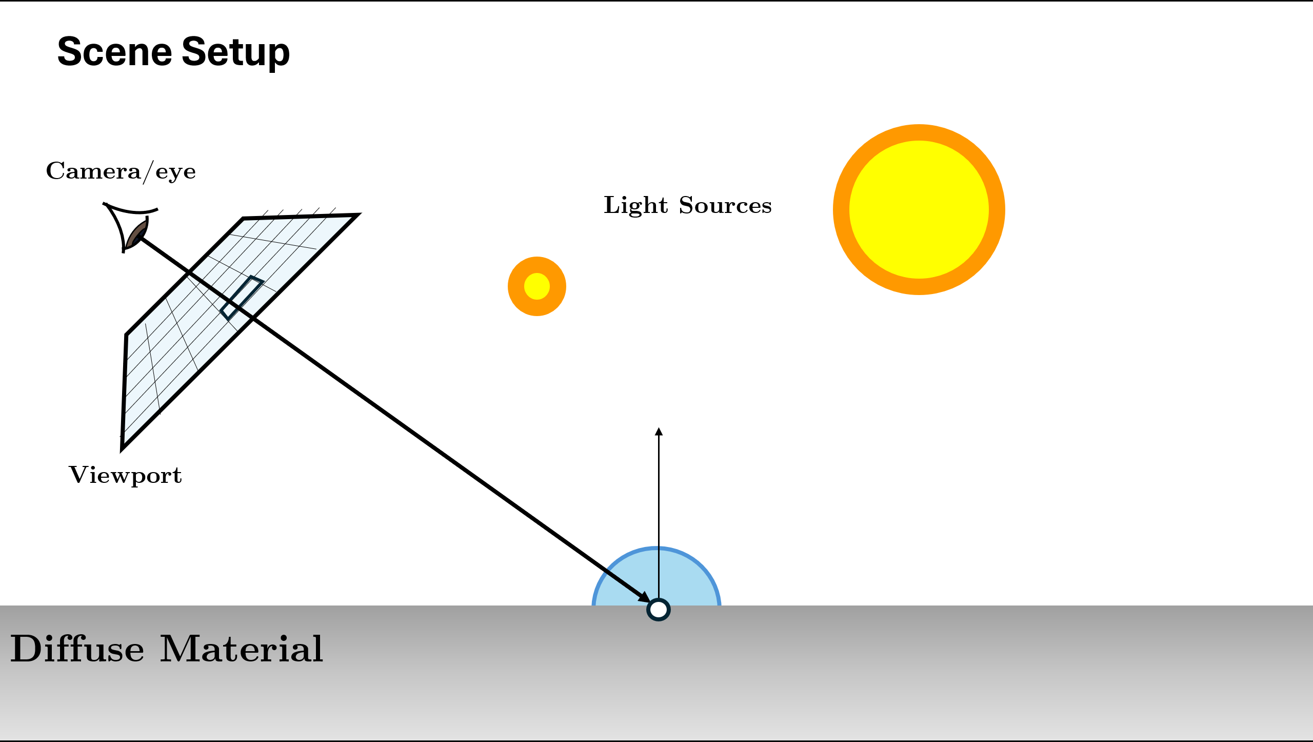
- Cameras: A camera model determines how and from where the scene is viewed, including how an image of the scene is recorded on a sensor. Many rendering systems generate viewing rays stating at the camera that are then traced into the scene to determine which objects are visible at each pixel.
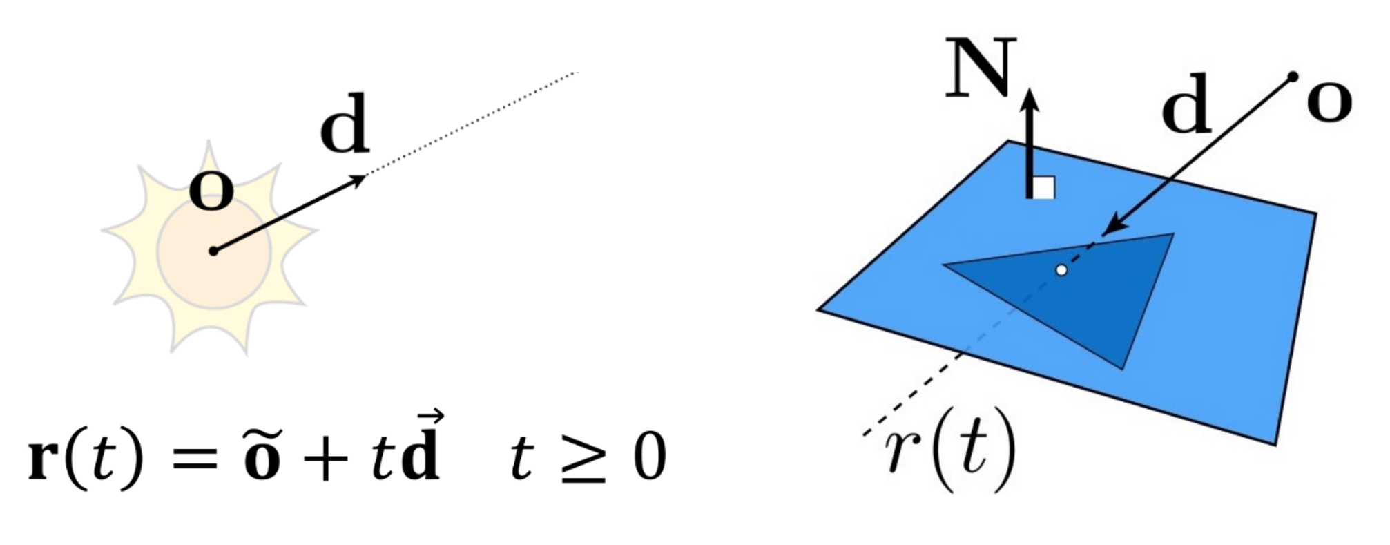
- Ray-object inetrsections: We must be able to tell precisely where a given ray intersects a given geometric object. In addition, we need to determine certain properties of the object at the intersection point, such as a surface normal or its material.
For the faster Ray-Triangle intersection, the BVH (Bounding Volumes Heirarchy) data-structure is usually used. A simplified visualization for it is given below:
Light Sources: Without lighting, there would be little point in rendering a scene. A ray tracer must model the distribution of light throughout the scene, including not only the locations of the lights themselves but also the way in which they distribute their energy throughout space.
Visibility: In order to know whether a given light deposits energy at a point on a surface, we must know whether there is an uninterrupted path from the point to the light source. Fortunately, this question is easy to answer in a ray tracer, since we can just construct the ray from the surface to the light, find the closest ray–object intersection, and compare the intersection distance to the light distance.
- Light scattering at surfaces: Each object must provide a description of its appearance, including information about how light interacts with the object’s surface, as well as the nature of the reradiated (or scattered) light. Models for surface scattering are typically parameterized so that they can simulate a variety of appearances.
Indirect light transport: Because light can arrive at a surface after bouncing off or passing through other surfaces, it is usually necessary to trace additional rays to capture this effect.
Ray propagation: We need to know what happens to the light traveling along a ray as it passes through space. If we are rendering a scene in a vacuum, light energy remains constant along a ray. Although true vacuums are unusual on Earth, they are a reasonable approximation for many environments. More sophisticated models are available for tracing rays through fog, smoke, the Earth’s atmosphere, and so on.
The Rendering Equation
At the heart of physically based rendering lies the Rendering Equation, introduced by James Kajiya (1986). It provides a unified mathematical framework describing how light is transferred and redistributed in a scene. Intuitively, it says that the radiance leaving a surface point in some direction is the sum of the light the surface emits and the light it reflects from all incoming directions.
Formally:
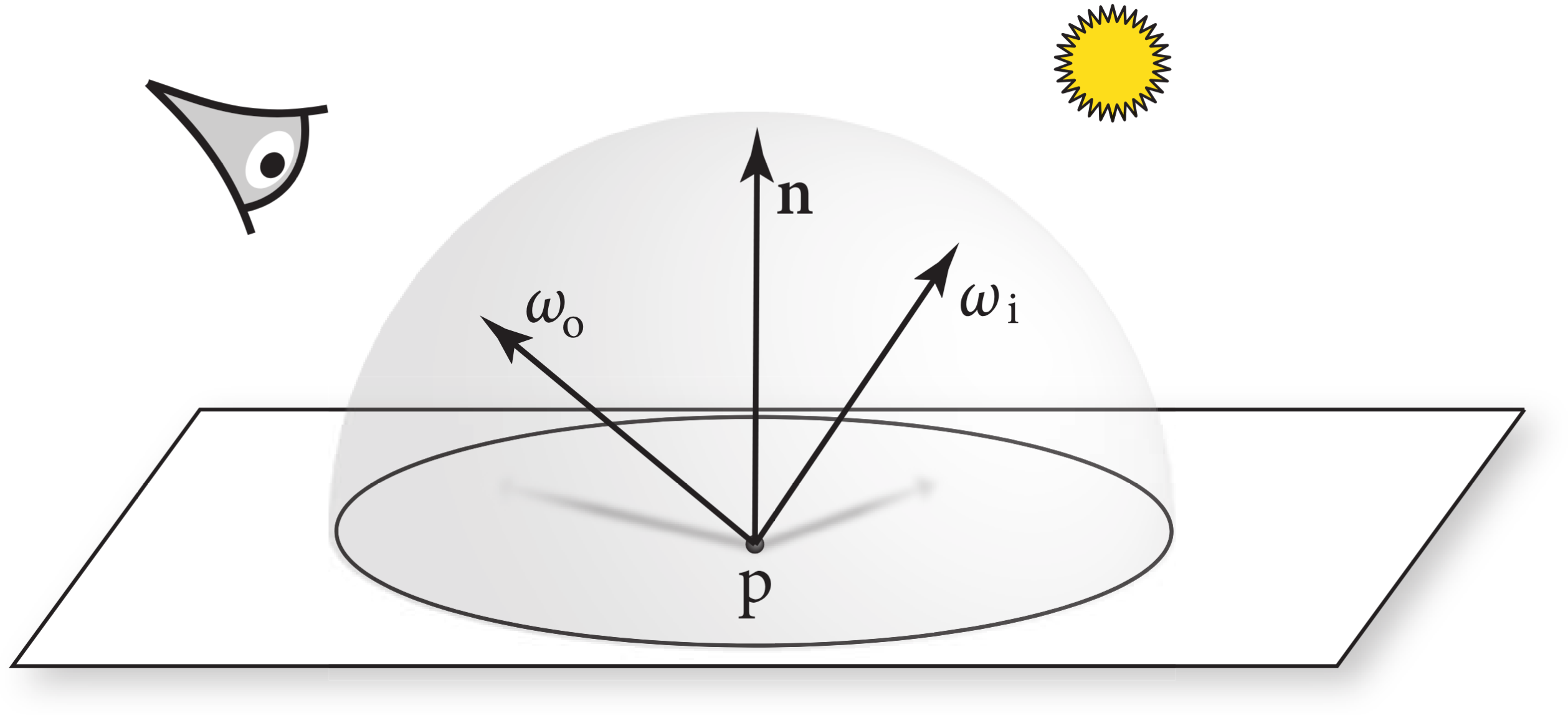
$$ L_o(x, \omega_o) = L_e(x, \omega_o) + \int_{\Omega} f_r(x, \omega_i, \omega_o)\; L_i(x, \omega_i)\; (\omega_i \cdot n)\; d\omega_i $$Where:
- $L_o(x, \omega_o)$ - outgoing radiance from point $x$ toward direction $\omega_o$ (what the camera sees).
- $L_e(x, \omega_o)$ - emitted radiance from $x$ (non-zero if $x$ is a light source).
- $f_r(x, \omega_i, \omega_o)$ - BRDF (Bidirectional Reflectance Distribution Function): fraction of light from direction $\omega_i$ scattered into $\omega_o$.
- $L_i(x, \omega_i)$ - incoming radiance arriving at $x$ from direction $\omega_i$.
- $(\omega_i \cdot n)$ - cosine foreshortening term (angle between incoming direction and surface normal $n$).
- $\Omega$ - hemisphere of directions above the surface.
Intuition
- The integral accumulates contributions from every incoming direction over the hemisphere.
- Because $L_i$ itself depends on outgoing radiance from other points, the equation is recursive - it captures global illumination (indirect lighting, caustics, etc.).
- Exact analytic solutions are generally impossible for complex scenes; we therefore rely on numerical approximation.
Path Tracing calculates an approximation for the rendering equation using Monte Carlo Integrals.
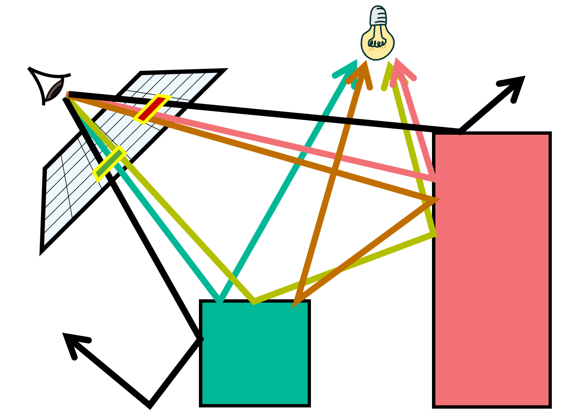
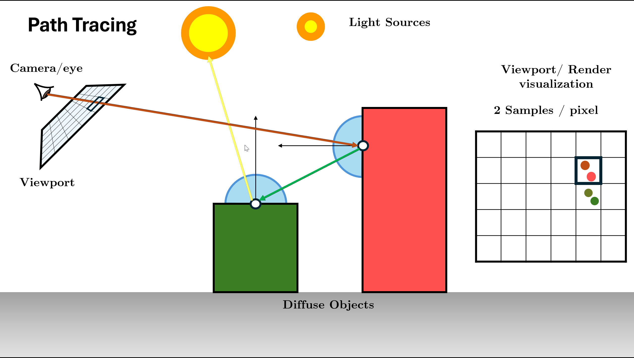
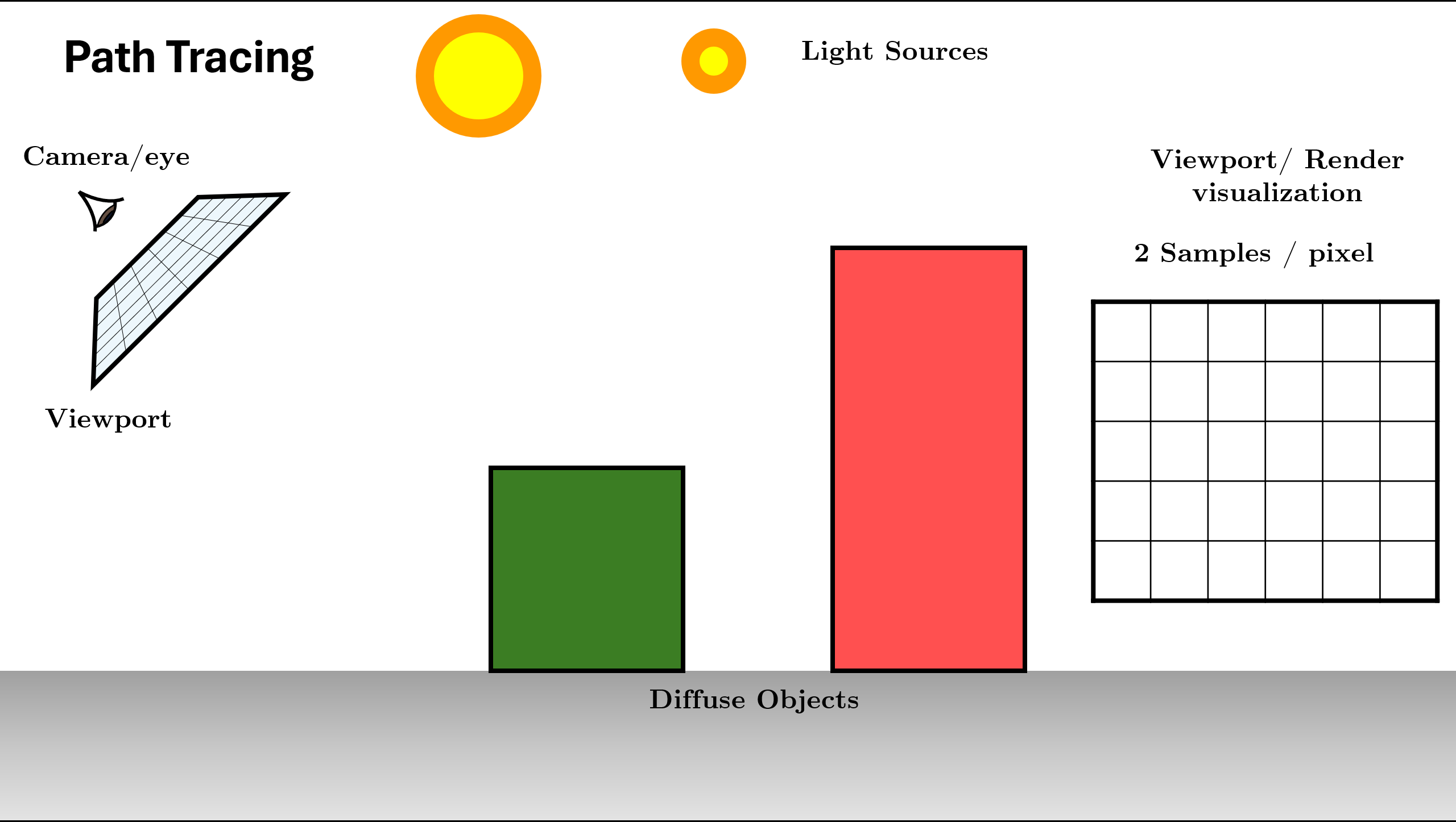
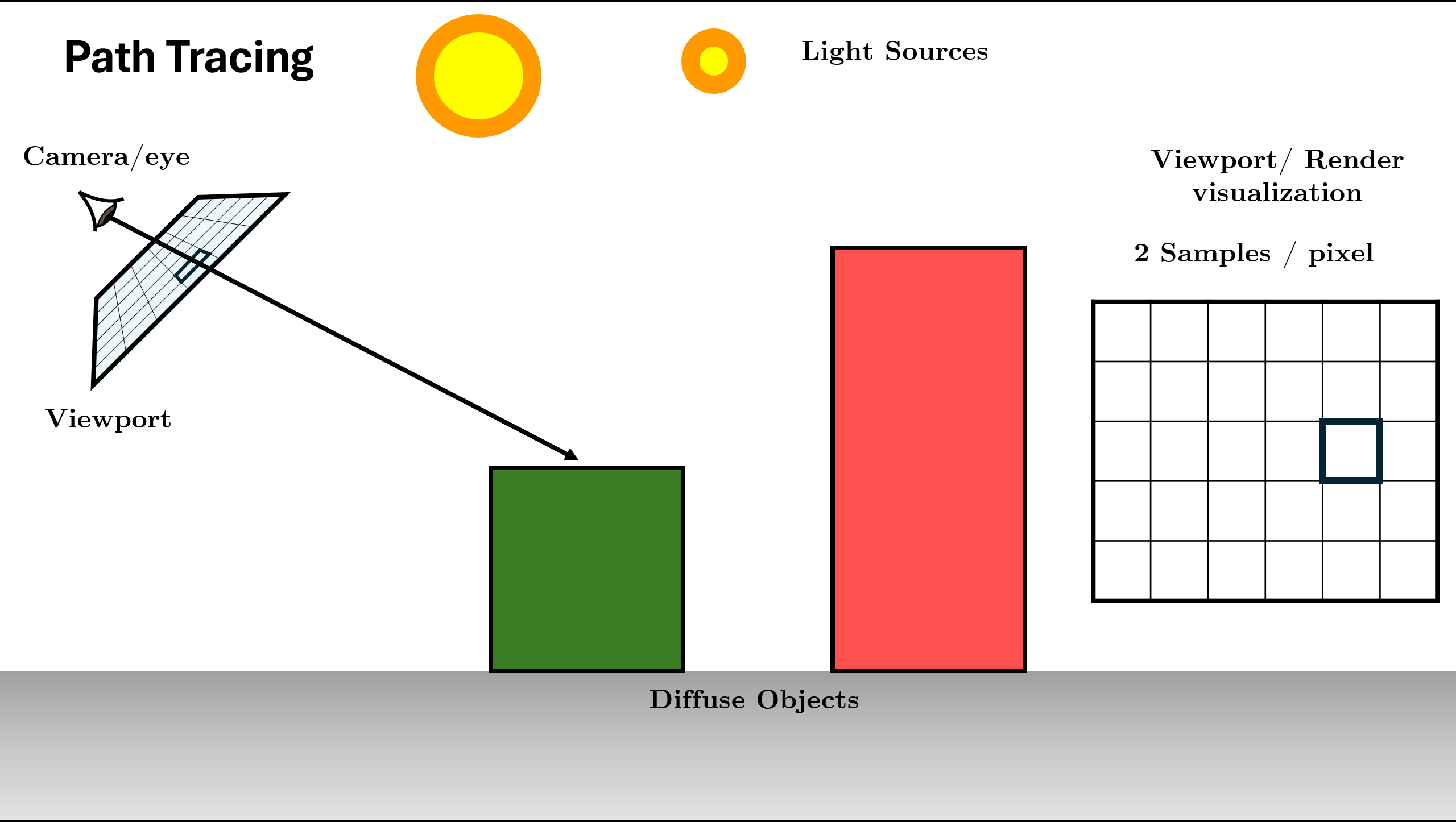
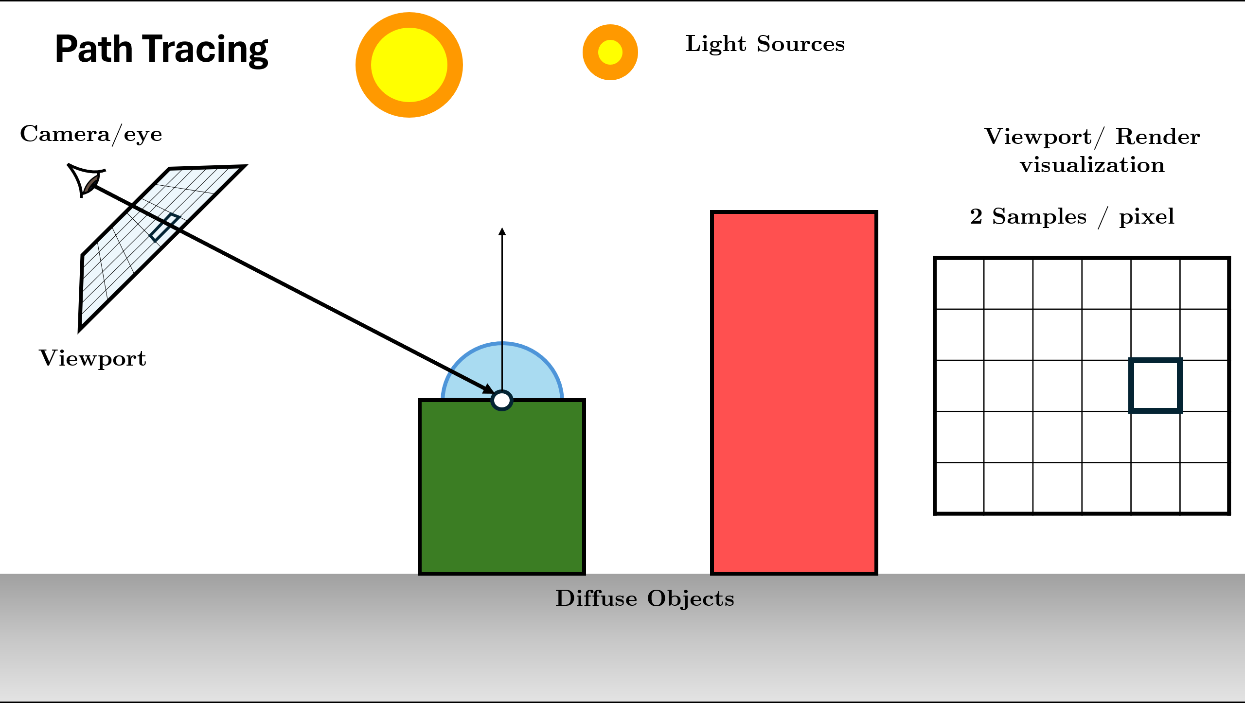
Rendering Equation Visualization
We can write this one big integral slightly differently as
$$ L(x\to v)=E_x+ \int_{\Omega} f_r \left( E_{x'} + \int_{\Omega'} f_r' \cdots \cos(\theta_{\omega'})\, d\omega' \right) \cos(\theta_{\omega})\, d\omega $$Which we can expand to get
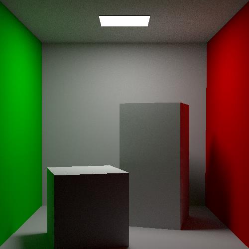
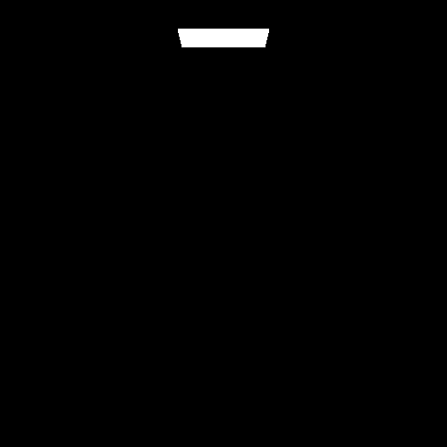
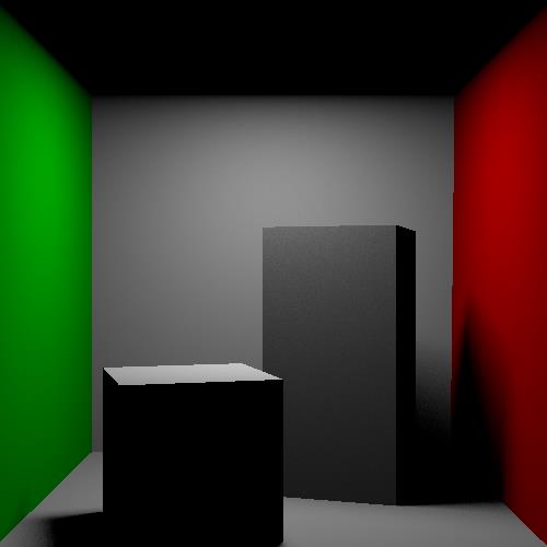
$$ \begin{aligned} L(x\to v) &= E_x \\ &\quad + \int_{\Omega} f_r\,E_{x'}\cos(\theta_{\omega})\,d\omega \\ &\quad + \int_{\Omega} f_r \int_{\Omega'} f_r'\,E_{x''}\cos(\theta_{\omega'})\cos(\theta_{\omega})\,d\omega'\,d\omega \\ &\quad + \int_{\Omega} f_r \int_{\Omega'} f_r' \int_{\Omega''} f_r''\,E_{x'''}\cos(\theta_{\omega''})\cos(\theta_{\omega'})\cos(\theta_{\omega})\,d\omega''\,d\omega'\,d\omega \\ &\quad + \cdots \end{aligned} $$After expanding the rendering integra, we can easily visualize the components of the integral and how they contribute to the final image
Alternate formualtions of the Rendering Equation
The following formulations can be found in Eric Veach’s PhD Thesis, or Tu Wien Rendering Course which I have used as resources.
Classic Surface Rendering Equation
First, this is the standard rendering equation we we’ll see in most local path guiding papers. It picks a direction of contribution and intergrates over all the direction of contribution (upper hemisphere / sphere). For a given direction, the radiance already includes all visible surfaces along that ray in that direction, so no explicit visibility term is needed.
$$ L_o(x, \omega_o) = L_e(x, \omega_o) + \int_{\Omega} f_r(x, \omega_i, \omega_o)\; L_i(x, \omega_i)\; (\omega_i \cdot n)\; d\omega_i $$Where:
- $L_o(x, \omega_o)$ - outgoing radiance from point $x$ toward direction $\omega_o$ (what the camera sees).
- $L_e(x, \omega_o)$ - emitted radiance from $x$ (non-zero if $x$ is a light source).
- $f_r(x, \omega_i, \omega_o)$ - BRDF (Bidirectional Reflectance Distribution Function): fraction of light from direction $\omega_i$ scattered into $\omega_o$.
- $L_i(x, \omega_i)$ - incoming radiance arriving at $x$ from direction $\omega_i$.
- $(\omega_i \cdot n)$ - cosine foreshortening term (angle between incoming direction and surface normal $n$).
- $\Omega$ - hemisphere of directions above the surface.
Surface Area (Geometry-Explicit) Rendering Equation
This is the same formulation with change of variables the difference being instead of picking direction, we explicitly take the contribution of whole scene by integrating over all the points on surface of the scene. To make sure the occluded parts are not accidentally counted Visibility term is added and for making it consistent with lambert’s cosine law, the geometry term is added.
$$ L_o(x, \omega_o) = L_e(x, \omega_o) + \int_{A} f_r(x, \omega_i, \omega_o)\; L_o(y, -\omega_i)\; G(x,y)\; V(x,y)\; dA_y $$Where:
- $A$ - set of all surfaces in the scene (integration domain).
- $y$ - surface point contributing light to $x$.
- $\omega_i$ - direction from $x$ to $y$.
- $L_o(y, -\omega_i)$ - outgoing radiance from $y$ toward $x$.
- $f_r(x, \omega_i, \omega_o)$ - BRDF at $x$.
- $G(x,y)$ - geometry term: $$ G(x,y) = \frac{(\omega_i \cdot n_x)(-\omega_i \cdot n_y)}{\|x - y\|^2} $$
- $V(x,y)$ - visibility function (1 if $x$ and $y$ are mutually visible, 0 otherwise).
- $dA_y$ - differential surface area at $y$.
Operator Form of the Rendering Equation
This, as the name suggests, treats the transport of light rays as operator. This formulation is useful for proofs of convergence, existence etc.
$$ L = L_e + \mathcal{T} L $$Where:
- $L$ - radiance function over all surface points and directions.
- $L_e$ - emitted radiance.
- $\mathcal{T}$ - light transport operator defined by: $$ (\mathcal{T}L)(x, \omega_o) =\int_{\Omega}f_r(x, \omega_i, \omega_o)\;L_i(x, \omega_i)\;(\omega_i \cdot n)d\omega_i $$
- Integration domain - hemisphere of directions above the surface.
This form emphasizes that global illumination is a fixed-point problem.
Solution operator
For simplicity of notation $L_e = E$. Rearrange:
$$L = E + \mathcal{T}L$$$$L - \mathcal{T}L = E$$$$(I - \mathcal{T})L = E$$So the formal solution is:
$$ L = (I - \mathcal{T})^{-1} E $$and $S$ is the solution operator
$$S = (I - \mathcal{T})^{-1} E$$Neumann-series expansion
Using the Neumann-series identity:
$$ (I-\mathcal{T} )^{-1} = I + \mathcal{T} + \mathcal{T}^2 + \mathcal{T}^3 + \cdots $$Substitute into the solution:
$$ \begin{aligned} L &= (I-\mathcal{T} )^{-1}E \\ &= (I + \mathcal{T} + \mathcal{T} ^2 + \mathcal{T} ^3 + \cdots)\,E \\ &= E + \mathcal{T}E + \mathcal{T}^2E + \mathcal{T}^3E + \cdots \end{aligned} $$The following visualizes the individual components (similar to the one given in the rendering equation) but with appropriate operator formulation for clarity.
The following visualizes the accumulation of individual components:
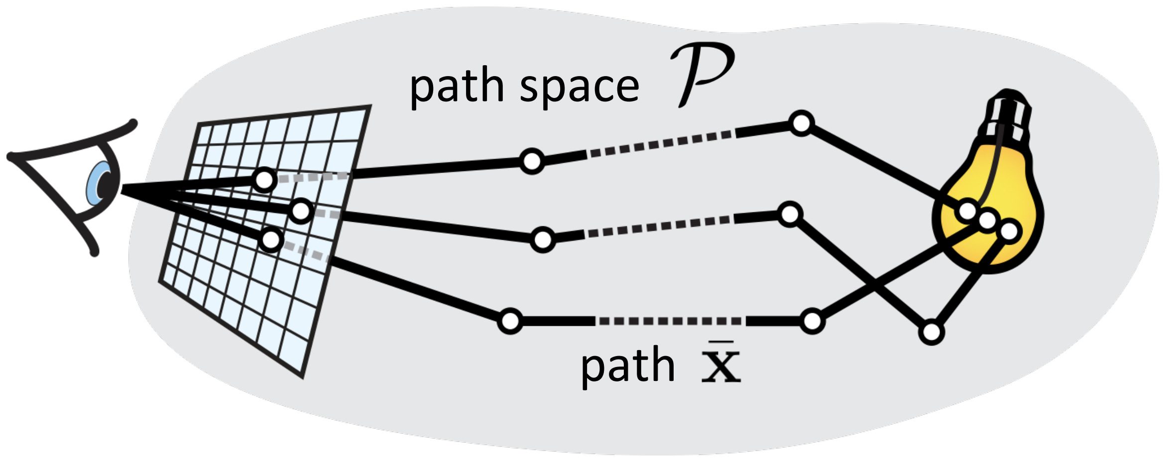
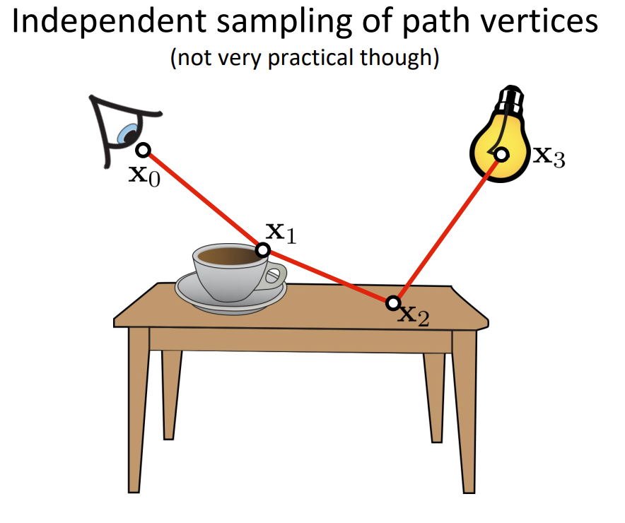
Path Integral Formulation of Light Transport
This formulation integrates over the domain of all light transport paths. This let’s us see the light transport as a contribution of different paths. This is very intuitive for the MC methods as it emphasies that different paths have different contribution and we are integrating over all possible path (or at least approximating that integral). This also makes is easy to see we can also work with “good” paths directly instead of choosing the ray direction in the classical one.
$$ I = \int_{\mathcal{P}} f(\bar{x})\; d\mu(\bar{x}) $$Where:
$$ f(\bar{x}) = L_e(x_0)\; \prod_{i=1}^{k} f_r(x_i)\; G(x_{i-1}, x_i)\; V(x_{i-1}, x_i) $$And:
- $\mathcal{P}$ - set of all possible light paths of all lengths $$ \bar{x} = (x_0, x_1, \ldots, x_k) \in \mathcal{P_k} $$ $$ \mathcal{P} = \bigcup_{k=1}^{\infty} \mathcal{P_k} $$ with vertices on surfaces or in volumes.
- $x_0$ - light source point.
- $x_k$ - point visible to the sensor.
- $f_r(x_i)$ - scattering function (BRDF/BSDF) at vertex $x_i$.
- $G(x_{i-1}, x_i)$ - geometry term between consecutive vertices.
- $V(x_{i-1}, x_i)$ - visibility term.
- $d\mu(\bar{x})$ - path-space measure (product of area, volume, and directional measures).
Visualizing Different Paths
We can see the interaction of light with Specular (S), Diffuse (D) objects. We can write all of the types of interaction of lights as regular expression $L(D | S)^*E$
The following sections contain the basics of probability required to knwo about how the Path Tracing is approximating the integral and ensuring the approximation is close enough to the actual solution. The sections are taken from online version of Intro to Probability, Statistics and Random Processes
Monte Carlo Basics
Because Monte Carlo integration is based on randomization, we’ll first discuss some ideas from probability and statistics.
First we define a random variable.
Definition - Random Variable
A random variable $X$ is a function that maps outcomes from the sample space $\Omega$ to the set of real numbers $\mathbb{R}$:
$$ X : \Omega \rightarrow \mathbb{R} $$Each outcome $\omega \in \Omega$ is assigned a numerical value $X(\omega)$, representing the realization of the random variable.
We also defined a Probability Mass Function. The probabilitues of events $\lbrace X=x_k \rbrace$ are formally shown by the probability mass function (PMF) of $X$.
Definition - Probability Mass Function
Let $X$ be a discrete Random variable with range $R_X=\lbrace x_1, x_2, \dots \rbrace$ (finite or countably infinite). The function:
$$ p_X(x_k) = P(X=x_k), \text{for k = }1, 2, \dots $$is called the probability mass function (PMF) of $X$
Thus, the PMF is a probability measure that gives us probabilities of the possible values for a random variable.
Properties - Probability Mass Function (PMF)
$$ \boxed{ \begin{aligned} &\text{Let } X \text{ be a discrete random variable with range } \mathcal{R}_X \text{ and PMF } p_X(x) = P(X = x). \\[6pt] &\text{Then the PMF satisfies the following properties:} \\[10pt] &1.\ \textbf{Non-negativity: } 0 \le p_X(x) \le 1, \quad \forall x \in \mathcal{R}_X \\[6pt] &2.\ \textbf{Normalization: } \sum_{x \in \mathcal{R}_X} p_X(x) = 1 \\[6pt] &3.\ \textbf{Additivity over sets: } P(X \in A) = \sum_{x \in A} p_X(x), \quad \forall A \subseteq \mathcal{R}_X \end{aligned} } $$The PMF is one way to describe the distribution of a discrete random variable and cannot be defined over continuous variabels. The cumulative distribution function (CDF) of a random variable is another method to describe the distribution of random variables. The advantage of the CDF is that it can be defined for any kind of random variable (discrete, continuous, and mixed).
Definition - Cumulative Distribution Function
The cumulative distribution function (CDF) of random variable $X$ is defined as :
$$F_X(x) = p(X\leq x_k), \text{for all }x\in\mathbb{R}$$$F_X$ is called the cumulative distribution function (CDF) of $X$
Note that the subscript $X$ indicates that this is the CDF of the random variable $X$. Also, note that the CDF is defined for all $x\in \mathbb{R}$
$$ \boxed{ \forall\, a \le b, \quad P(a < X \le b) = F_X(b) - F_X(a) } $$Definition - Probability Density Function (PDF)
Let $X$ be a continuous random variable. The probability density function (PDF) of $X$ is a non-negative function $f_X(x)$ satisfying:
$$ P(a \le X \le b) = \int_a^b f_X(x)\,dx $$for all real numbers $a \le b$.
The PDF must satisfy the following properties:
$$ \boxed{ \begin{aligned} &1.\ \textbf{Non-negativity: } f_X(x) \ge 0, \quad \forall x \in \mathbb{R} \\[4pt] &2.\ \textbf{Normalization: } \int_{-\infty}^{\infty} f_X(x)\,dx = 1 \end{aligned} } $$Unlike a PMF, the PDF itself does not give probabilities directly; instead, the probability that $X$ lies in an interval is given by the area under $f_X(x)$ over that interval.
Definition - Expected Value
Let $X$ be a continuous random variable with probability density function $f_X(x)$.
$$ \boxed{ \mathbb{E}[X] = \int_{-\infty}^{\infty} x\, f_X(x)\, dx } $$
The expected value (or mean) of $X$, denoted by $\mathbb{E}[X]$, is defined as:
The expected value represents the theoretical average value of $X$ - the value one would obtain as the limit of the sample mean if the random process were repeated infinitely many times.
Definition - Variance
Let $X$ be a continuous random variable with probability density function $f_X(x)$ and expected value $\mu = \mathbb{E}[X]$.
$$ \boxed{ \mathrm{Var}(X) = \int_{-\infty}^{\infty} (x - \mu)^2\, f_X(x)\, dx } $$
The variance of $X$, denoted by $\mathrm{Var}(X)$, measures the expected squared deviation of $X$ from its mean:Equivalently, variance can also be expressed as:
$$ \boxed{ \mathrm{Var}(X) = \mathbb{E}[X^2] - (\mathbb{E}[X])^2 } $$
The variance quantifies the spread or dispersion of the distribution - larger values indicate greater variability of $X$ around its mean.
The Monte Carlo Estimator
Let $I$ be an integral of interest (the rendering equation for us), defined over $\Omega$:
$$ I = \int_{\Omega} f(x)\, dx $$where $\Omega$ is any reasonable integration domain.
From Integration to Expectation
The key insight of Monte Carlo integration is recognizing that any integral can be rewritten as an expectation of a random variable.
Given a probability density function (PDF) $p(x)$ defined over $\Omega$, we can decompose the integral as:
$$ I = \int_{\Omega} f(x)\, dx = \int_{\Omega} \frac{f(x)}{p(x)} p(x)\, dx $$By the definition of expected value for a continuous random variable $X$ with PDF $p(x)$:
$$ \mathbb{E}[g(X)] = \int_{\Omega} g(x) \cdot p(x)\, dx $$we can identify:
$$ I = \mathbb{E}\left[\frac{f(X)}{p(X)}\right] $$where $X$ is a random variable drawn from distribution $p(x)$.
Properties of the $p(x)$ in MC Estimator
The PDF $p(x)$ must satisfy the following fundamental properties:
$$ \boxed{ \begin{aligned} &1.\ \textbf{Non-negativity:}\quad p(x) \geq 0, \quad \forall x \in \Omega \\[8pt] &2.\ \textbf{Normalization:}\quad \int_{\Omega} p(x)\, dx = 1 \\[8pt] &3.\ \textbf{Support condition:}\quad p(x) > 0 \text{ wherever } f(x) \neq 0 \end{aligned} } $$The third property is crucial: if $p(x) = 0$ at some point where $f(x) \neq 0$, the ratio $\frac{f(x)}{p(x)}$ becomes undefined or infinite, making the estimator invalid.
Definition - Monte Carlo Estimator
To approximate the expected value $\mathbb{E}[f(X)/p(X)]$, we draw $N$ independent samples $X_1, X_2, \ldots, X_N$ from $p(x)$ and compute their average:
$$ \boxed{ \hat{I}_{MC} = \frac{1}{N}\sum_{i=1}^{N} \frac{f(X_i)}{p(X_i)}, \quad X_i \stackrel{\text{i.i.d.}}{\sim} p(x) } $$This is the importance sampling Monte Carlo estimator. The term “importance sampling” refers to the fact that we sample proportionally to how important each region is to the integral (weighted by $p(x)$).
Derivation of Properties
Property 1: Unbiasedness
To prove that $\mathbb{E}[\hat{I}_{MC}] = I$, we take the expectation of both sides:
$$ \mathbb{E}[\hat{I}_{MC}] = \mathbb{E}\left[\frac{1}{N}\sum_{i=1}^{N} \frac{f(X_i)}{p(X_i)}\right] $$By linearity of expectation:
$$ = \frac{1}{N}\sum_{i=1}^{N} \mathbb{E}\left[\frac{f(X_i)}{p(X_i)}\right] $$Since each $X_i \sim p(x)$ independently and identically, each term equals the same expectation:
$$ = \frac{1}{N}\sum_{i=1}^{N} \int_{\Omega} \frac{f(x)}{p(x)} \cdot p(x)\, dx $$$$ = \frac{1}{N}\sum_{i=1}^{N} \int_{\Omega} f(x)\, dx $$$$ = \frac{1}{N} \cdot N \cdot I = I $$Therefore:
$$ \boxed{\mathbb{E}[\hat{I}_{MC}] = I} $$The estimator is unbiased, meaning its expected value equals the true integral.
Property 2: Variance Derivation
The variance of the estimator is:
$$ \text{Var}(\hat{I}_{MC}) = \text{Var}\left(\frac{1}{N}\sum_{i=1}^{N} \frac{f(X_i)}{p(X_i)}\right) $$Using the property that $\text{Var}(cY) = c^2 \text{Var}(Y)$ for constant $c$:
$$ = \frac{1}{N^2} \text{Var}\left(\sum_{i=1}^{N} \frac{f(X_i)}{p(X_i)}\right) $$Since the $X_i$ are independent, variances of independent random variables add:
$$ = \frac{1}{N^2} \sum_{i=1}^{N} \text{Var}\left(\frac{f(X_i)}{p(X_i)}\right) $$Each term has the same variance since all $X_i$ are identically distributed:
$$ = \frac{1}{N^2} \cdot N \cdot \text{Var}\left[\frac{f(X_1)}{p(X_1)}\right] $$$$ \boxed{\text{Var}(\hat{I}_{MC}) = \frac{1}{N}\text{Var}\left[\frac{f(X)}{p(X)}\right]} $$Property 3: Convergence Rate and Standard Error
The standard deviation (standard error) of the estimator is:
$$ \sigma(\hat{I}_{MC}) = \sqrt{\text{Var}(\hat{I}_{MC})} = \frac{1}{\sqrt{N}}\sqrt{\text{Var}\left[\frac{f(X)}{p(X)}\right]} $$$$ \boxed{\sigma(\hat{I}_{MC}) = \mathcal{O}\left(\frac{1}{\sqrt{N}}\right)} $$This means the error decreases proportionally to $N^{-1/2}$, independent of the dimensionality of the problem. This is a major advantage over deterministic numerical integration methods, which suffer from the “curse of dimensionality.”
Key observation: The error decreases as $\mathcal{O}\left(\frac{1}{\sqrt{N}}\right)$, so to reduce standard deviation by a factor of 4, we need 16 times more samples.
Summary: Properties of the Monte Carlo Estimator
$$ \boxed{ \begin{aligned} &\text{1. Unbiasedness:}\quad \mathbb{E}[\hat{I}_{MC}] = I \\[8pt] &\text{2. Variance:}\quad \text{Var}(\hat{I}_{MC}) = \frac{1}{N}\text{Var}\left[\frac{f(X)}{p(X)}\right] \\[8pt] &\text{3. Convergence:}\quad \text{Error} = \mathcal{O}(N^{-1/2}) \\[8pt] &\text{4. Standard Error:}\quad \sigma(\hat{I}_{MC}) \propto \frac{1}{\sqrt{N}} \end{aligned} } $$These properties make Monte Carlo integration particularly attractive for high-dimensional problems like rendering, where evaluating the rendering equation requires integrating over many dimensions (directions, wavelengths, time, etc.).
Importance Sampling
A natural question arises: what choice of $p(x)$ minimizes the variance? This is crucial because:
$$ \text{Var}(\hat{I}_{MC}) = \frac{1}{N}\text{Var}\left[\frac{f(X)}{p(X)}\right] $$The variance depends directly on how we choose $p(x)$. Can we choose $p(x)$ to make it smaller?
Variance of the Weighted Function
Let’s expand the variance term:
$$ \text{Var}\left[\frac{f(X)}{p(X)}\right] = \mathbb{E}\left[\left(\frac{f(X)}{p(X)}\right)^2\right] - \left(\mathbb{E}\left[\frac{f(X)}{p(X)}\right]\right)^2 $$The second term is fixed (it equals $I^2$, the integral we’re trying to compute). So to minimize variance, we need to minimize:
$$ \mathbb{E}\left[\left(\frac{f(X)}{p(X)}\right)^2\right] = \int_{\Omega} \frac{f(x)^2}{p(x)^2} \cdot p(x)\, dx = \int_{\Omega} \frac{f(x)^2}{p(x)}\, dx $$The Optimal Choice: p(x) ∝ f(x)
Claim: The variance is minimized when $p(x)$ is proportional to $f(x)$.
Let’s assume:
$$ p^*(x) = \frac{|f(x)|}{\int_{\Omega} |f(x)|\, dx} = \frac{|f(x)|}{I} $$where $I = \int_{\Omega} |f(x)|\, dx$ (assuming $f(x) \geq 0$ for simplicity).
What happens to the weighted ratio?
$$ \frac{f(X)}{p^*(X)} = \frac{f(X)}{f(X)/I} = I \quad \text{(constant!)} $$Since $\frac{f(X)}{p^*(X)}$ is a constant:
$$ \text{Var}\left[\frac{f(X)}{p^*(X)}\right] = \text{Var}[I] = 0 $$This is the best possible case: zero variance!
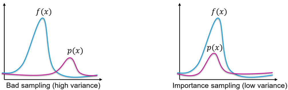
Why This Makes Intuitive Sense
When $p(x) \propto f(x)$:
- Regions where $f(x)$ is large: We sample frequently, so each sample contributes significant information
- Regions where $f(x)$ is small: We sample rarely, which is fine because they don’t contribute much anyway
- Result: Every sample carries roughly equal “importance” to the integral
By contrast, with uniform sampling $p(x) = \text{constant}$:
- We waste samples in regions where $f(x) \approx 0$ (unimportant)
- We don’t sample enough where $f(x)$ is large (important)
- The ratio $\frac{f(X)}{p(X)}$ varies wildly, causing high variance
Practical Reality: The Catch
While optimal importance sampling with $p(x) \propto f(x)$ is theoretically perfect, it’s impractical:
$$ p^*(x) = \frac{f(x)}{\int_{\Omega} f(x)\, dx} $$To construct this PDF, we already need to compute the integral we’re trying to find! This is circular.
In practice, we approximate: Choose $p(x)$ to be proportional to $f(x)$ as best we can:
- In path tracing: $p(x)$ might be proportional to the BRDF and lighting
- In neural importance sampling: Use neural networks to learn $p(x) \approx f(x)$
The better our approximation $p(x) \approx c \cdot f(x)$, the lower the variance.
The Importance Sampling Principle
$$ \boxed{ \begin{aligned} &\text{Best choice:}\quad p(x) \propto f(x) \Rightarrow \text{Var} = 0 \text{ (ideal)}\\[8pt] &\text{General principle:}\quad \text{Var} \propto \int_{\Omega} \frac{f(x)^2}{p(x)}\, dx\\[8pt] &\text{Practical strategy:}\quad \text{Choose } p(x) \text{ to approximate } f(x) \\[8pt] &\qquad\qquad\text{Better approximation} \Rightarrow \text{Lower variance} \Rightarrow \text{Fewer samples needed} \end{aligned} } $$This is why importance sampling is so powerful: by choosing $p(x)$ wisely, we can dramatically reduce the number of samples needed to achieve a target accuracy.
What are we sampling?
Now we know the theory of the importance sampling, the question is what is the importance sampling PDF $p(x)$ when we are solving the rendering equation. Based on the formulations of the rendering equation
Using the Classic Surface Rendering Equation, we can use a PDF $p(x)$ on the next direction $\omega_i$. So we will be calculating the estimate of the rendering integral using the Monte Carlo Methods by sampling the next direction using this formulation.
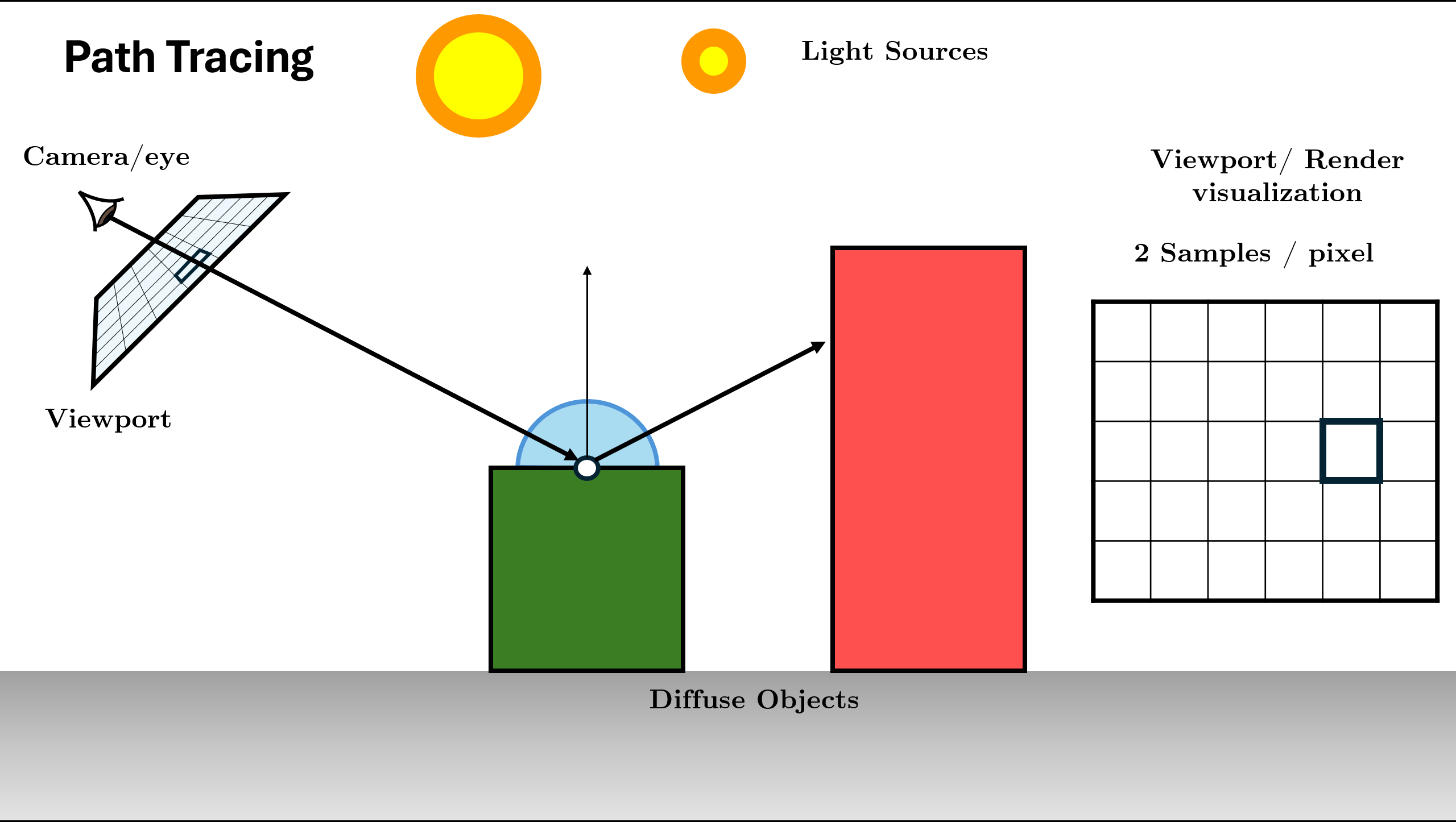
Path Tracing
Path Tracing is a rendering algorithm in computer graphics that simulates how light interacts with objects and participating media to generate realistic (physically plausible) images.This is conceptually a simple algorithm; it is based on following th path of a ray of light through a scene as it interacts with and bounces off objects in an environment.
It is an unbiased estimate of the rendering equation:
$$ L_o(x, \omega_o) = L_e(x, \omega_o) + \int_{\Omega} \boxed{f_r(x, \omega_i, \omega_o)\;}L_i(x, \omega_i)\; (\omega_i \cdot n)\; d\omega_i $$BxDF Functions
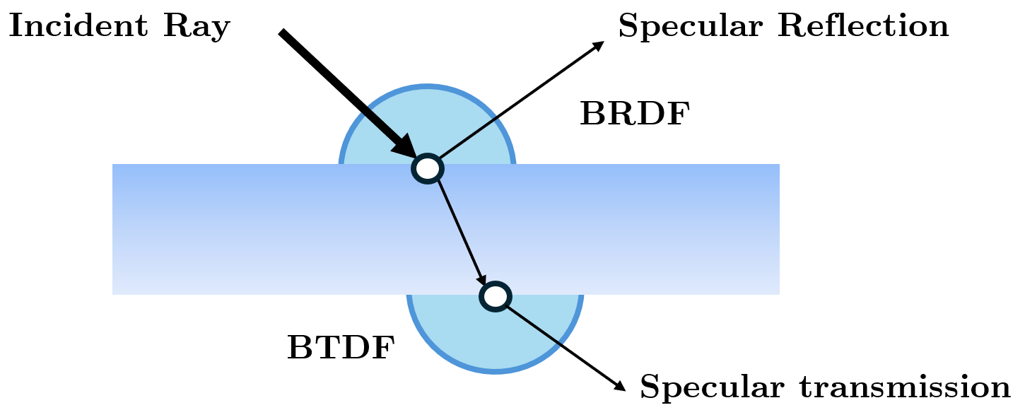
The concept behind all BxDF functions could be described as a black box with the inputs being any two angles, one for incoming (incident) ray and the second one for the outgoing (reflected or transmitted) ray at a given point of the surface. The output of this black box is the value defining the ratio between the incoming and the outgoing light energy for the given couple of angles
(BSDF) Bidirectional Scattering Distribution Function accounts for the light transport properties of the hit material. BSDF is a superset and the generalization of the BRDF and BTDF
BRDF (Bidirectional Reflectance Distribution Function) considers only the reflection of incoming light onto a surface
BTDF (Bidirectional transmittance distribution function) is similar to BRDF but for the opposite side of the surface when it is transmitted through the surface
(Some tend to use the term BSDF simply as a category name covering the whole family of BxDF functions.)
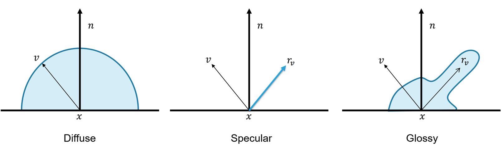
We usually distinguish three basic material types:
- Perfectly diffuse (light is scattered equally in/from all directions)
- Perfectly specular (light is reflected in/from exactly one direction)
- Glossy (mixture of the other two, specular highlights)
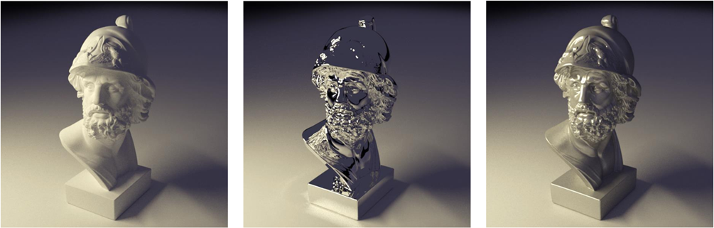
Now that we know about the BxDF functions which define the material properties, we can look at some example BSDF taken from Mitsuba renderer.
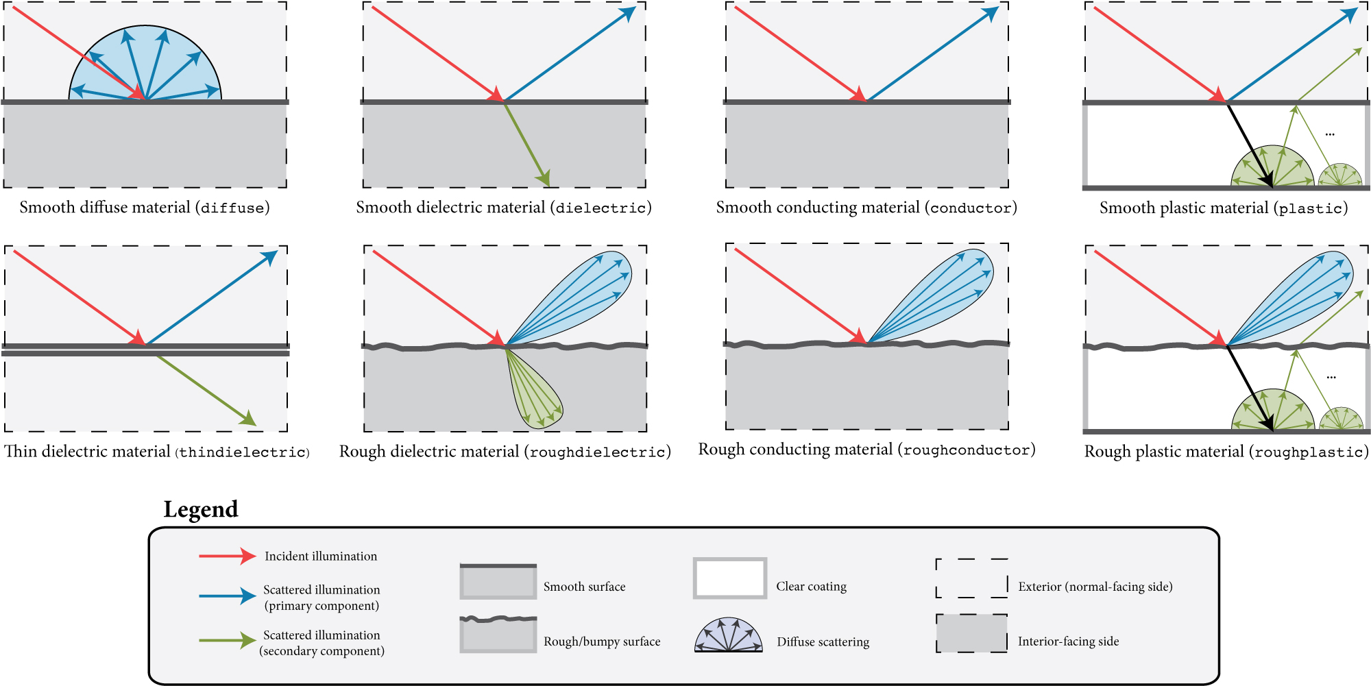
More details on BSDF can be found on Mitsuba 3 BSDF Plugins or at PBRT Reflection models.
We can also visualize how they look on hemisphere by using the interactive visualization below. This visualization uses baked bsdf for some materials in the Mitsuba 3 over a hemisphere.
Mapping (Hemi)Sphere to Grid
As the distribition is on a sphere/hemispehre, when using some methods the hemipshere is mapped to a grid which is then predicted by the guiding method. The grid can be discrete/continuous based on methods, but some of the methods for converion are:
Path Tracing Algorithm Steps (Recursive)
Generate camera ray through pixel using sensor
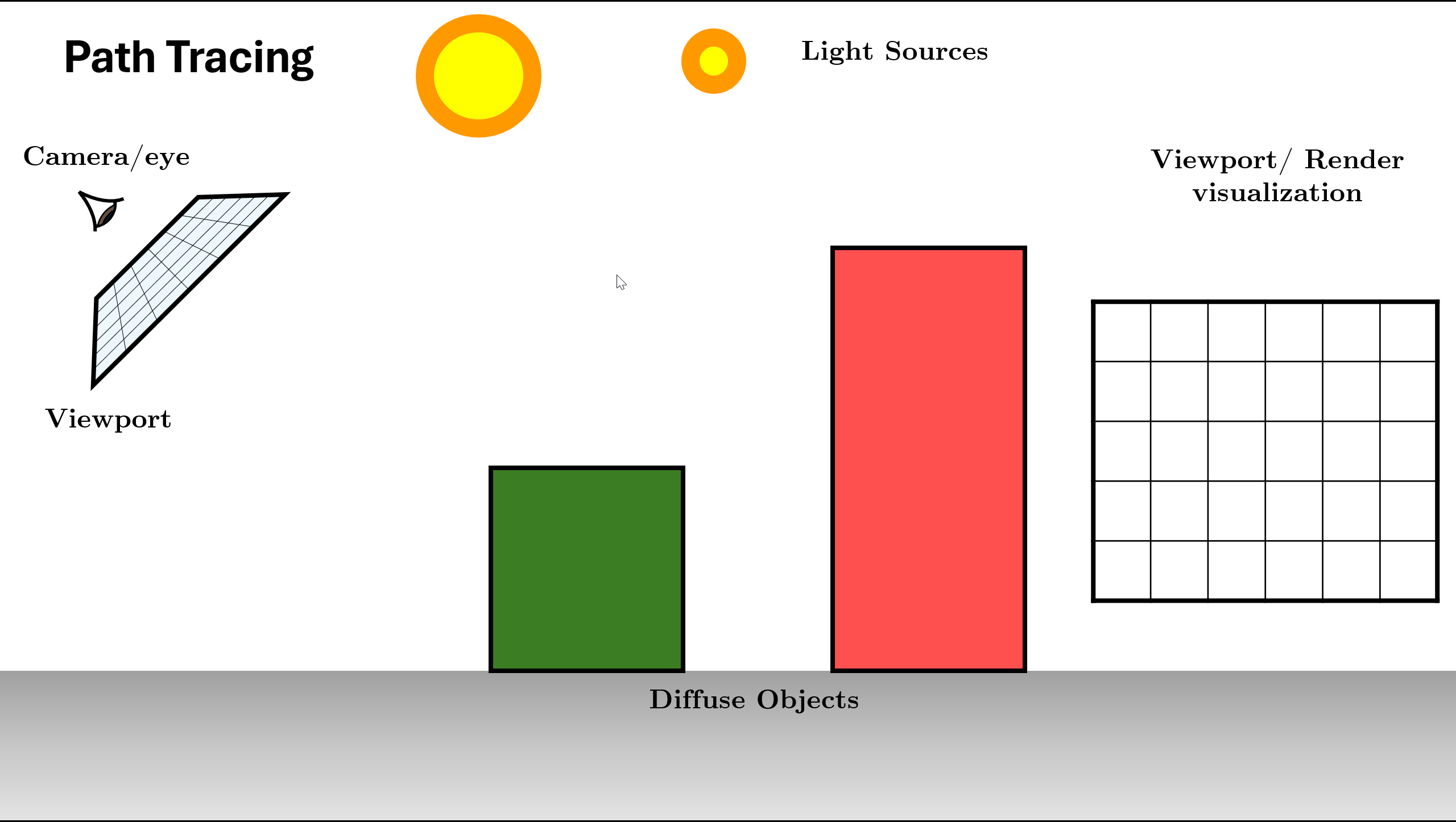
Figure 12. Initialize Scene and Generate Rays using Sensor Trace ray into scene, find nearest intersection. (If miss: return background).
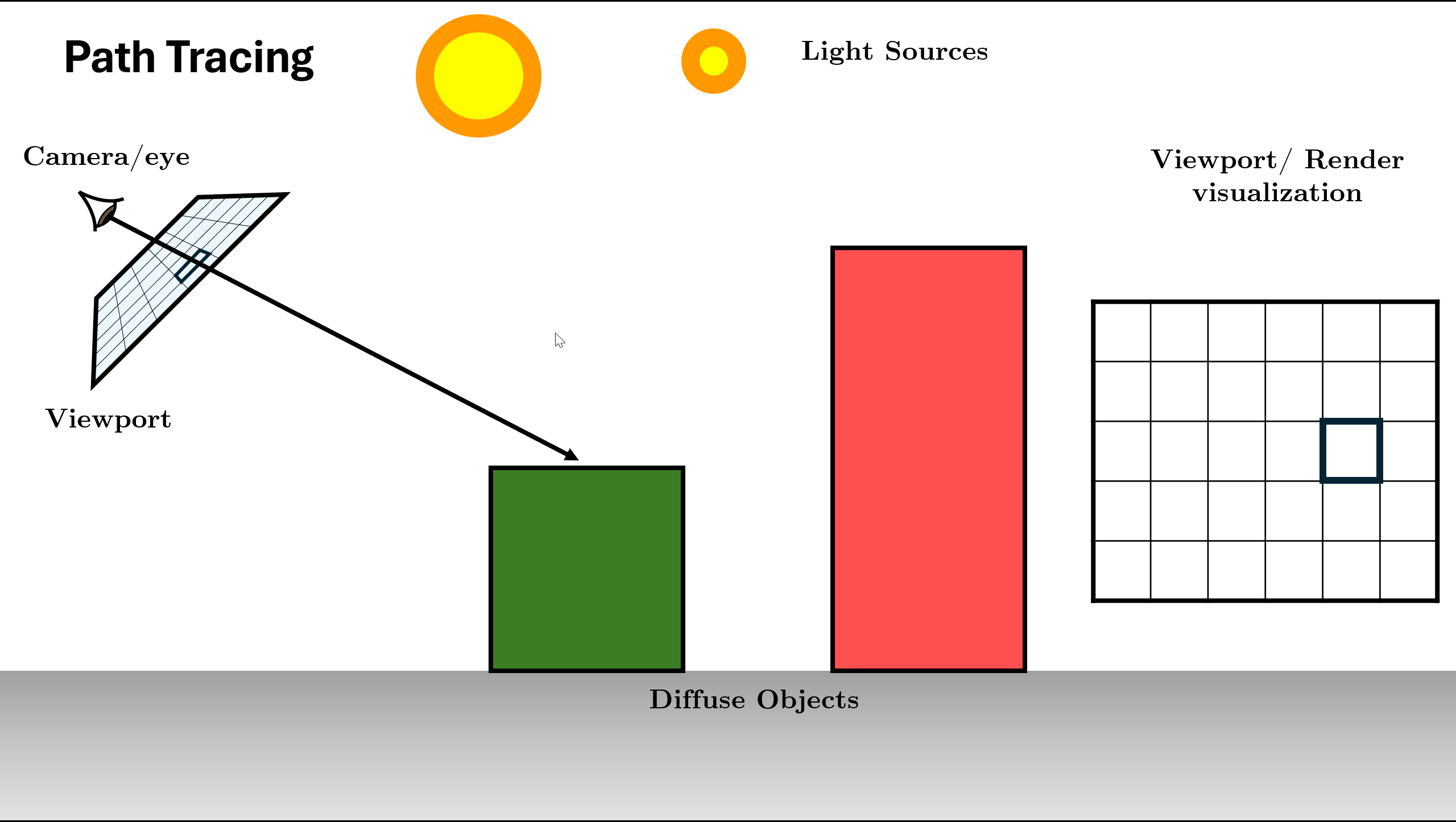
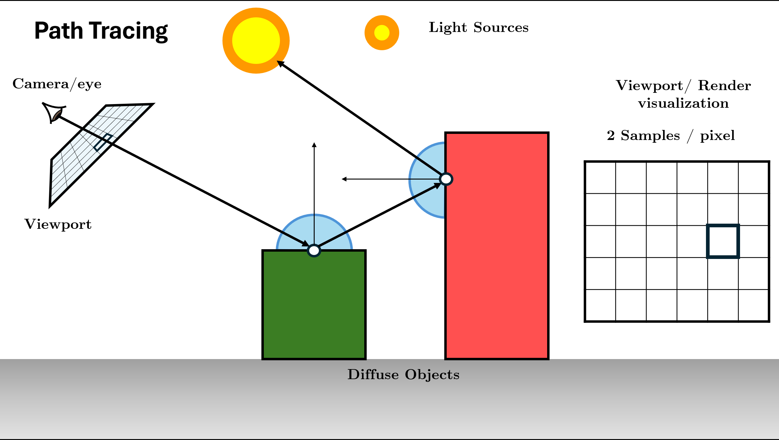
Figure 13. Trace Ray and Find Intersection (Base Case Check) Initialize Radiance ($L$) with surface emission ($L_e$) and Direct Light (NEE).
Sample BSDF to choose next direction and calculate Throughput (color).
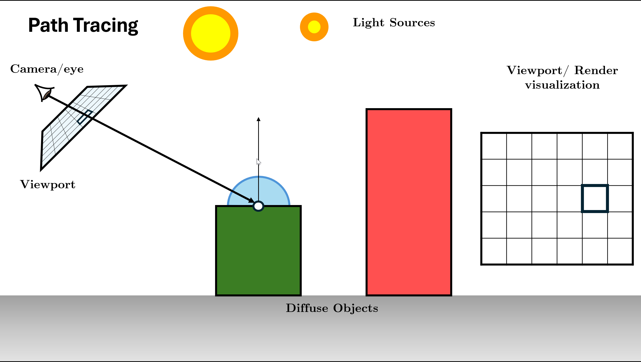
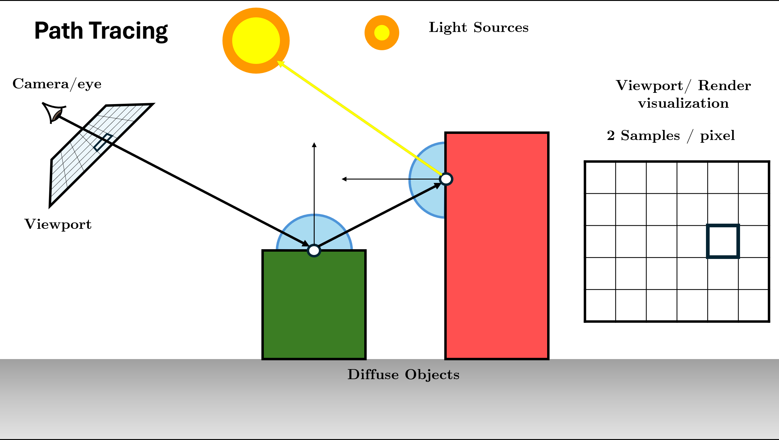
Figure 14. Query BSDF and calculate throughput (BSDF * Cos / PDF) Recursive Call: Spawn new ray and call
Trace()function for it.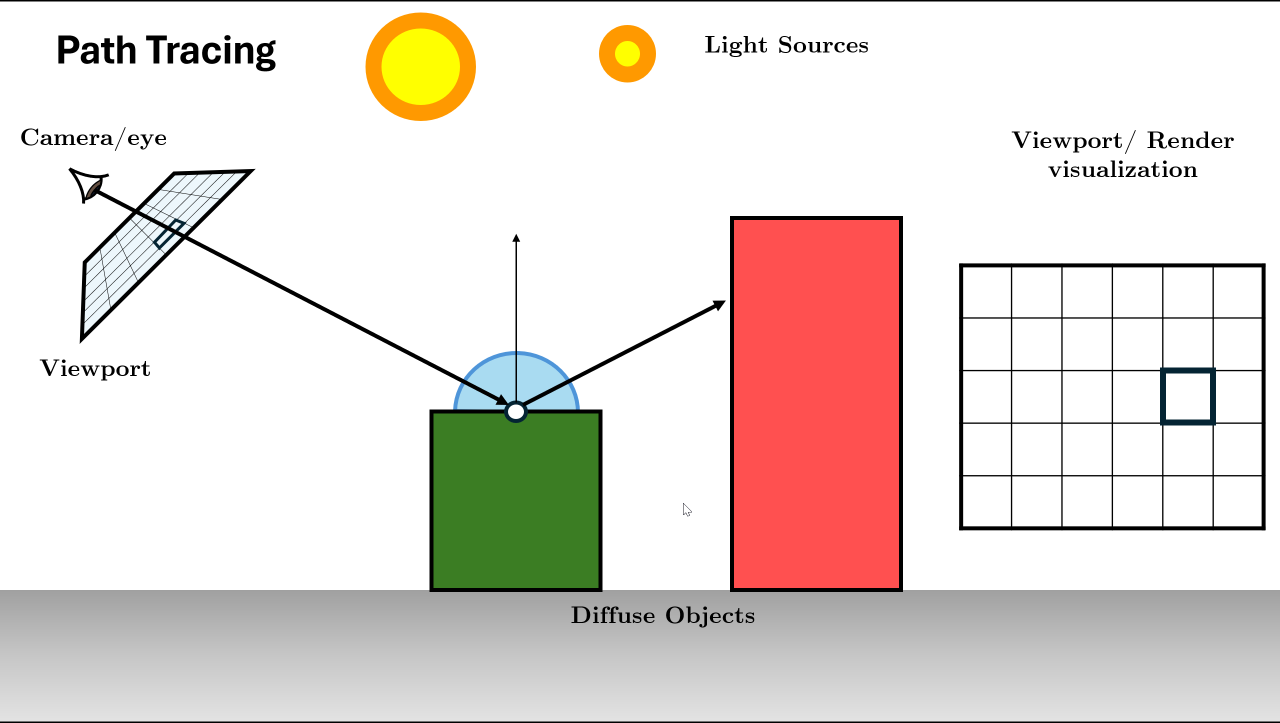
Figure 15. Spawn ray and recurse: L_in = Trace(new_ray)Recursion Depth: The function continues calling itself until max depth or Russian Roulette termination.
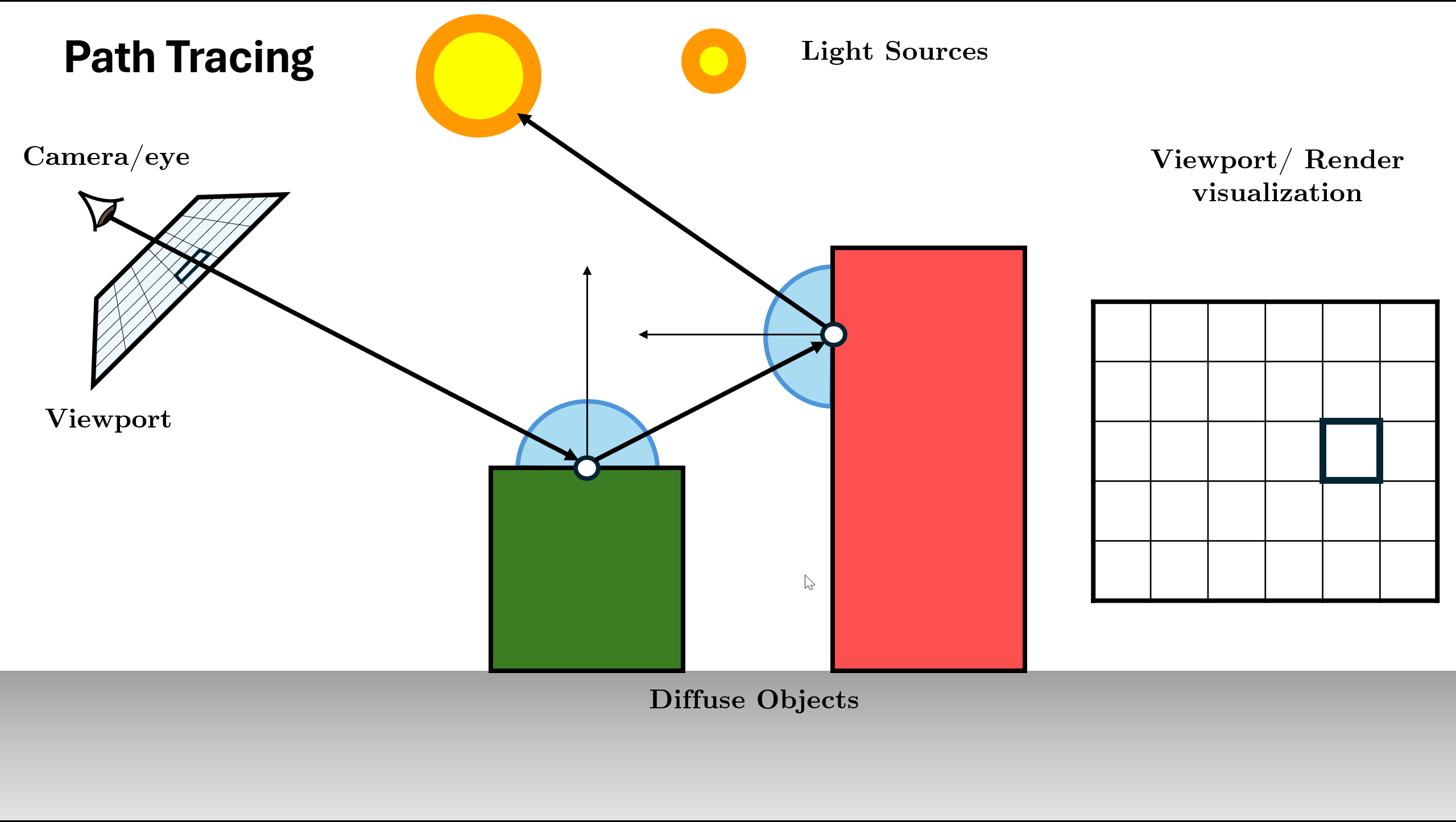
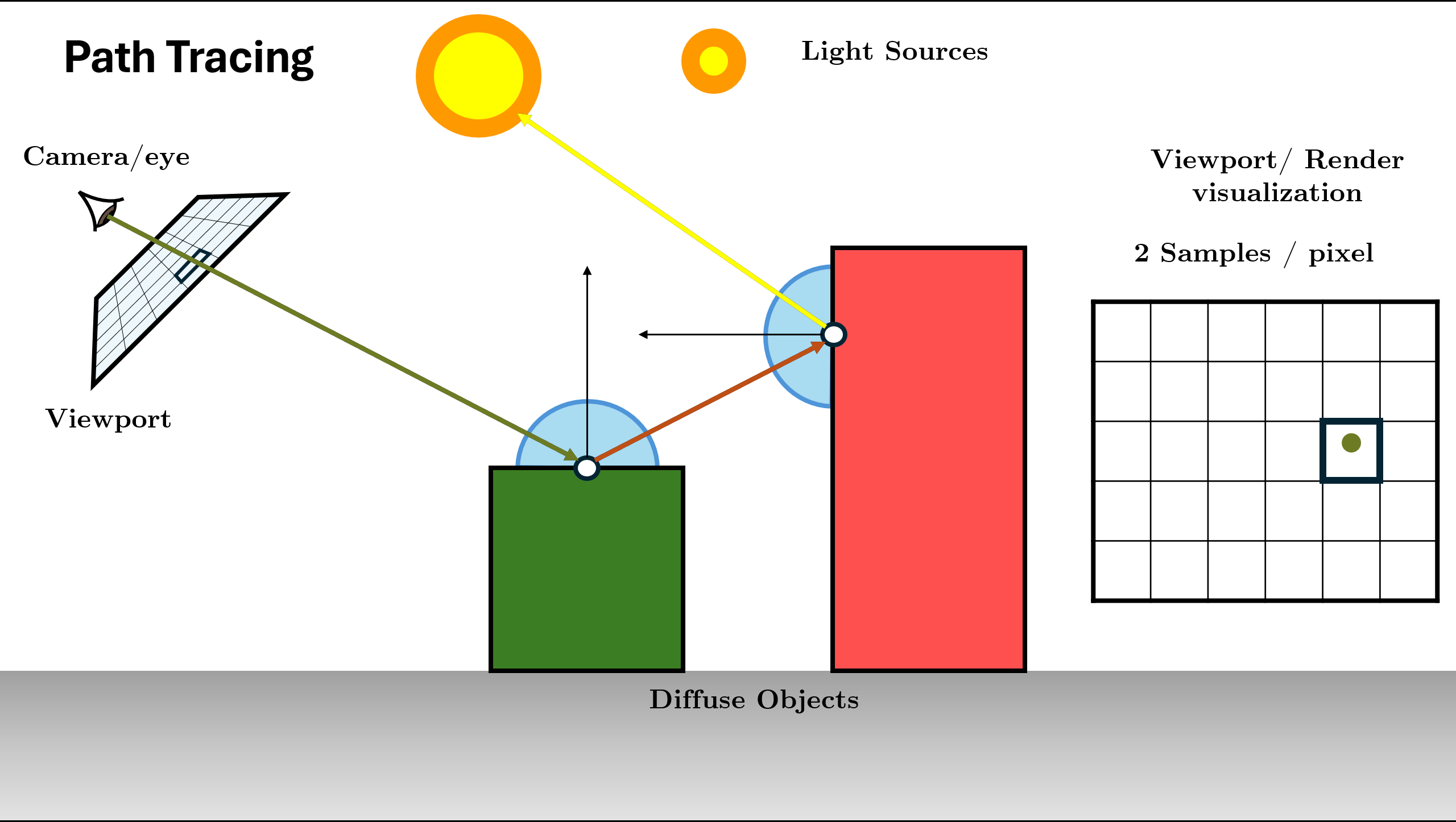
Figure 16. Recursion continues (Logic repeats for new ray) Return Total Radiance: Add indirect light to local emission ($L_e + \text{Throughput} \times L_{in}$) and return result.

Figure 17. Return combined radiance up the stack
Repeat the above process for all pixels (parallely as this is embarrasingly parallel) for some amount of samples per pixel
Path Tracing Steps Overview


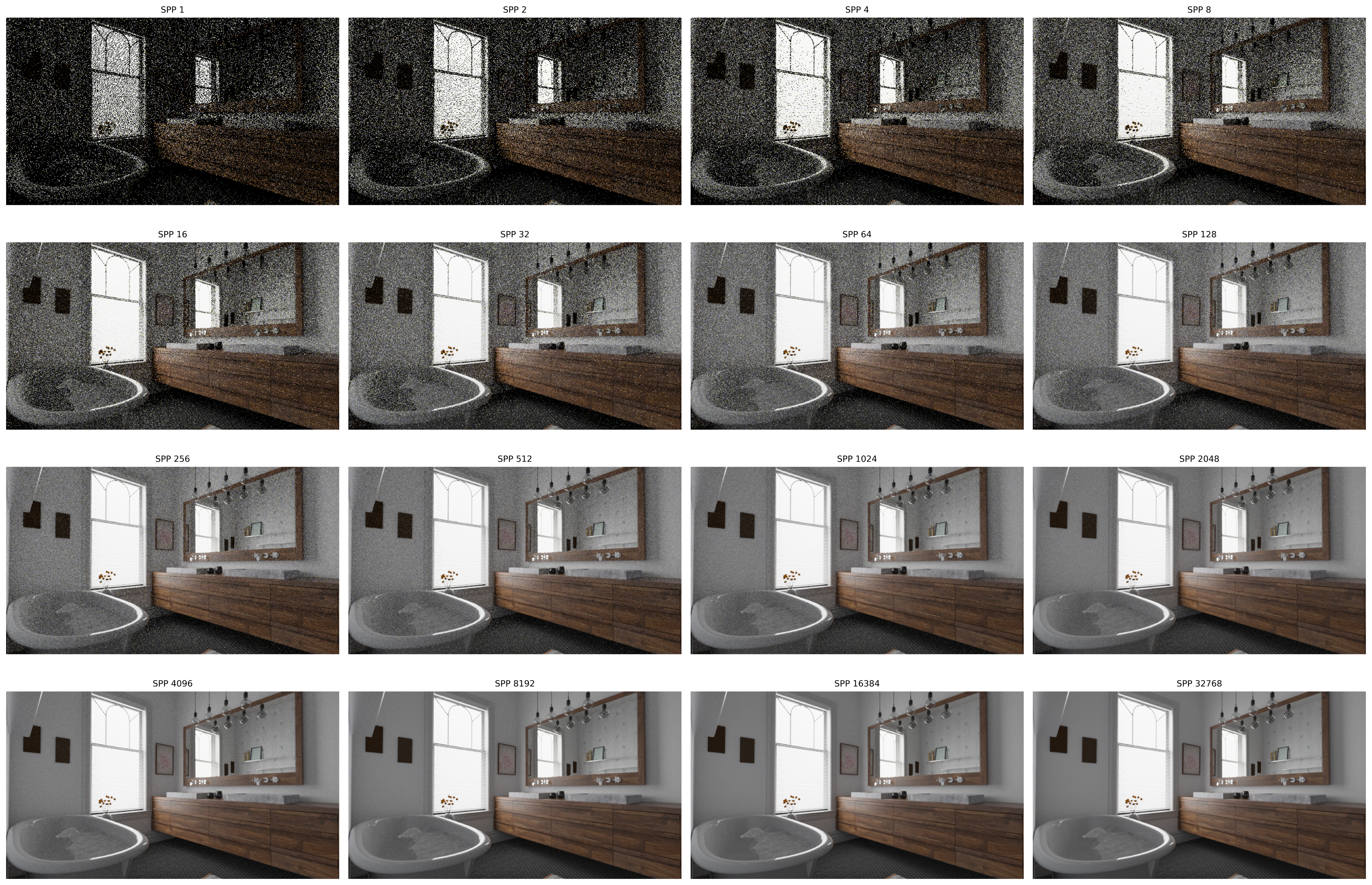
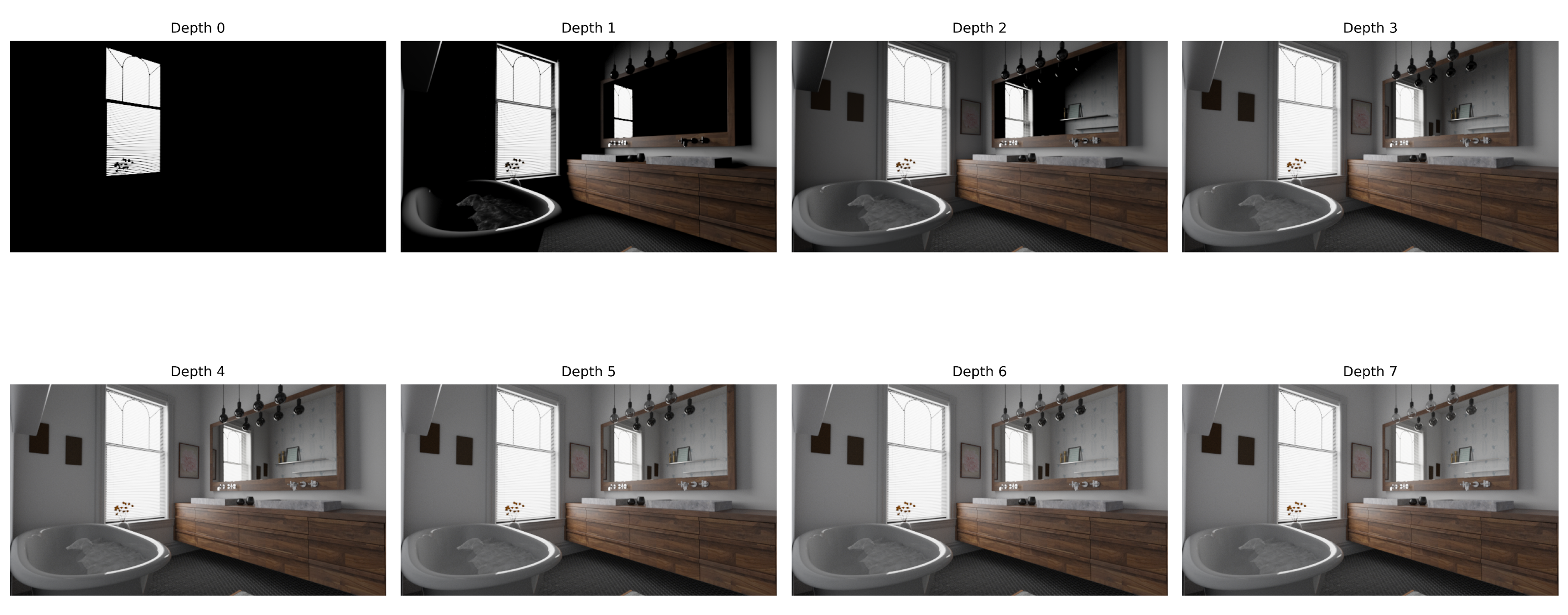
Interactive Ray Tracer Visualization
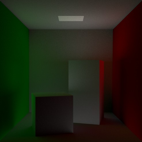
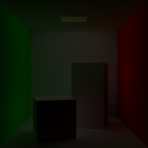
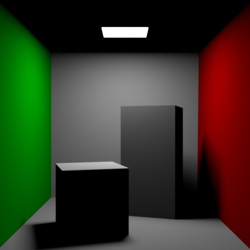
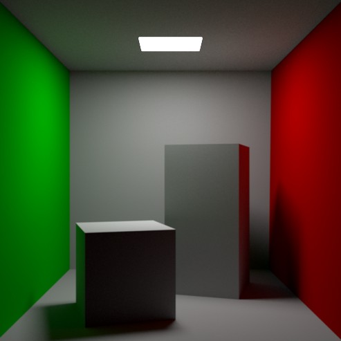
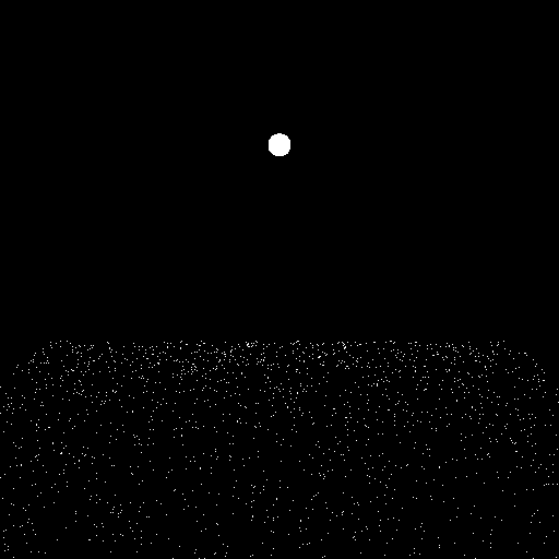
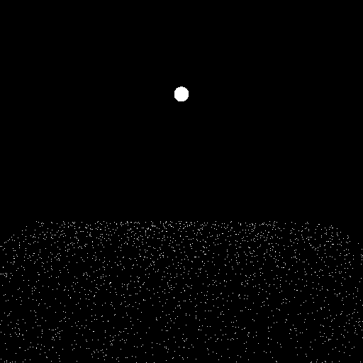
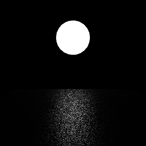
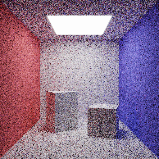
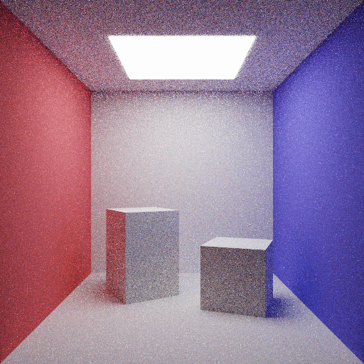
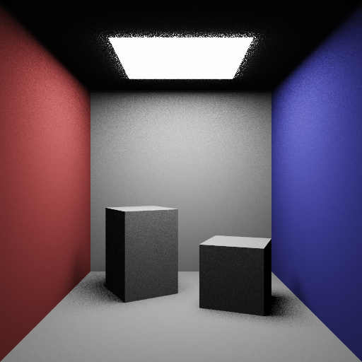
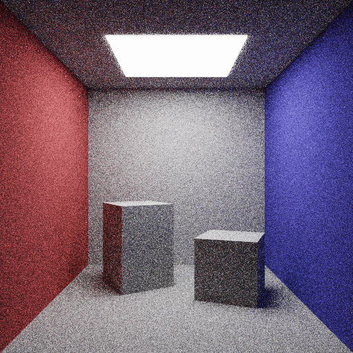
To show a real example, we can see the effects of Max Depth and Samples per pixes in the renders below. All of them are rendered using the PBRT renderer.
Recursive and Iterative Formulations
| Symbol | Meaning |
|---|---|
| $f$ | Throughput - cumulative product of BSDF and PDF terms: $f = \prod_{k=1}^{\text{depth}} \frac{f_r^{(k)}}{p_i^{(k)}}$ |
| $L$ | Accumulated radiance along the path |
| $L_e$ | Emitted radiance at surface intersection |
| $\omega_i$ | Sampled direction from BSDF distribution |
| $f_r$ | BSDF value: $f_r(x, \omega_i, \omega_o)$ |
| $p_i$ | PDF of sampled direction |
| $q$ | Russian roulette survival probability |
Input: scene, ray, depth, $\text{max\_depth}$, $\text{rr\_depth}$
Output: Radiance $L_o(x, \omega_o)$
Recursive Formulation
function PATHTRACE(scene, ray, depth)
    if depth ≥ max_depth then
        return 0
    end if

    si ← INTERSECT(ray, scene)
    if ¬si.valid() then
        return 0
    end if

    Lₑ ← si.bsdf.emission(ωₒ)
    (ωᵢ, fᵣ, p_ωᵢ) ← BSDF-SAMPLE(si.bsdf, ωₒ)

    next_ray ← RAY(si.p, ωᵢ)
    Lᵢ ← PATHTRACE(next_ray, depth + 1)
    Lᵣ ← (fᵣ · Lᵢ) / p_ωᵢ

    if depth ≥ rr_depth then
        q ← max(Lᵣ.r, Lᵣ.g, Lᵣ.b)
        if RAND() > q then
            return Lₑ
        end if
        Lᵣ ← Lᵣ / q
    end if

    return Lₑ + Lᵣ
end function
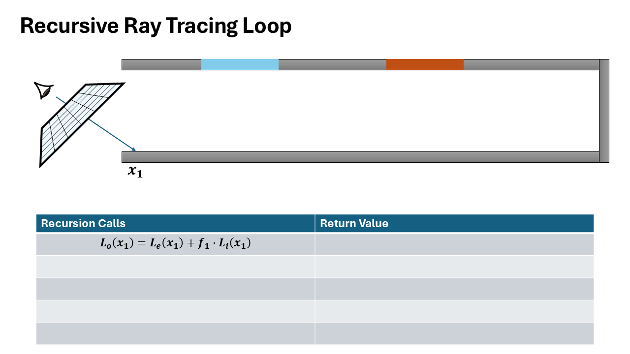
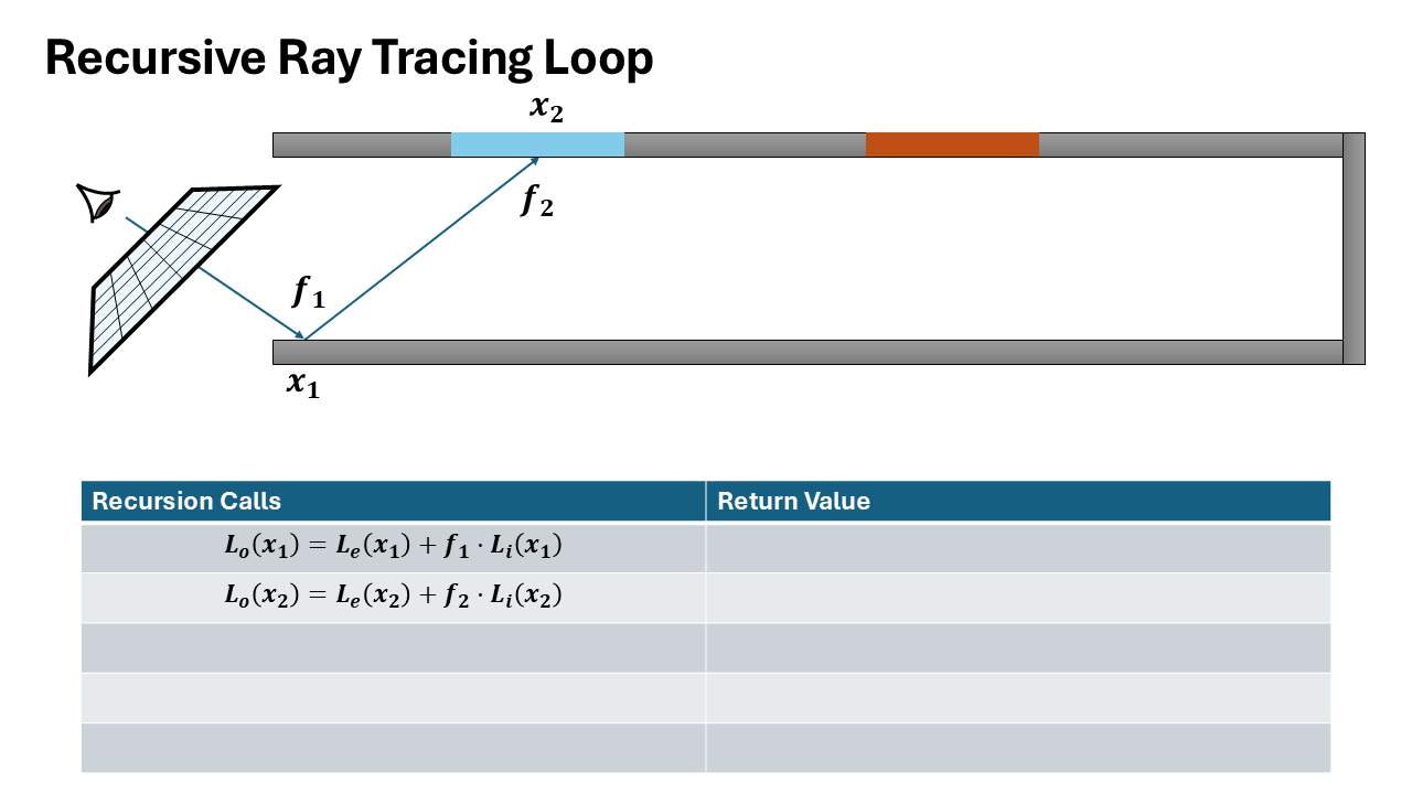
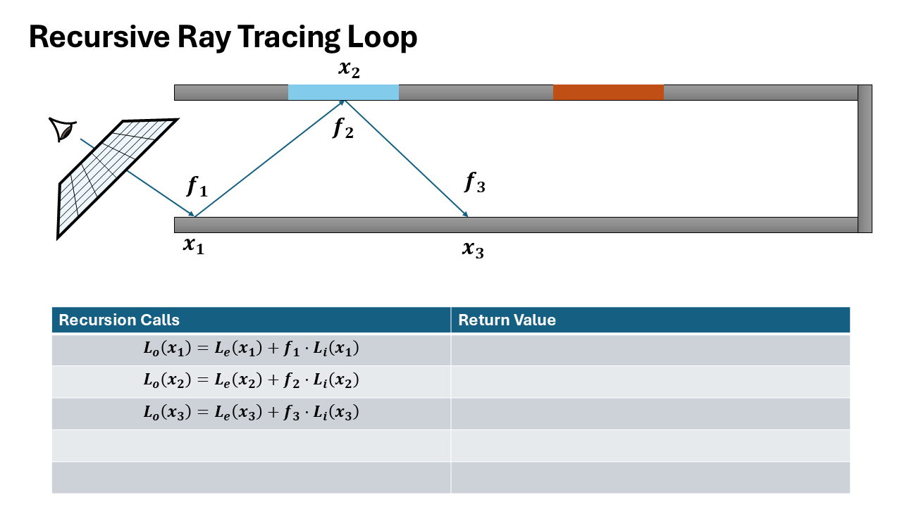
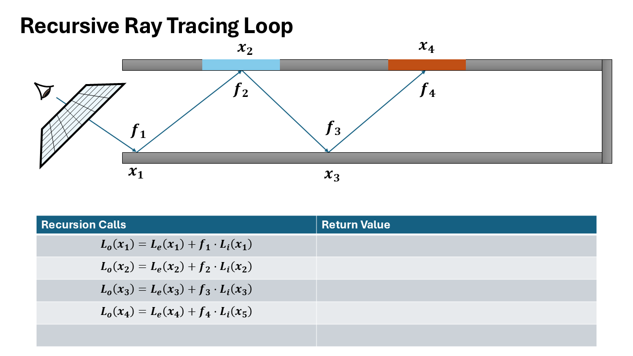
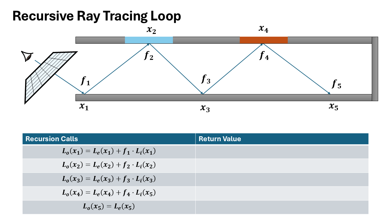
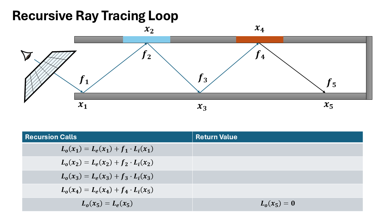
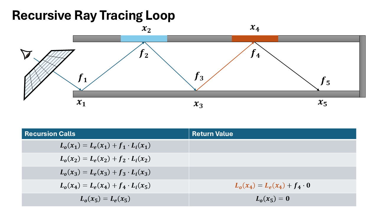
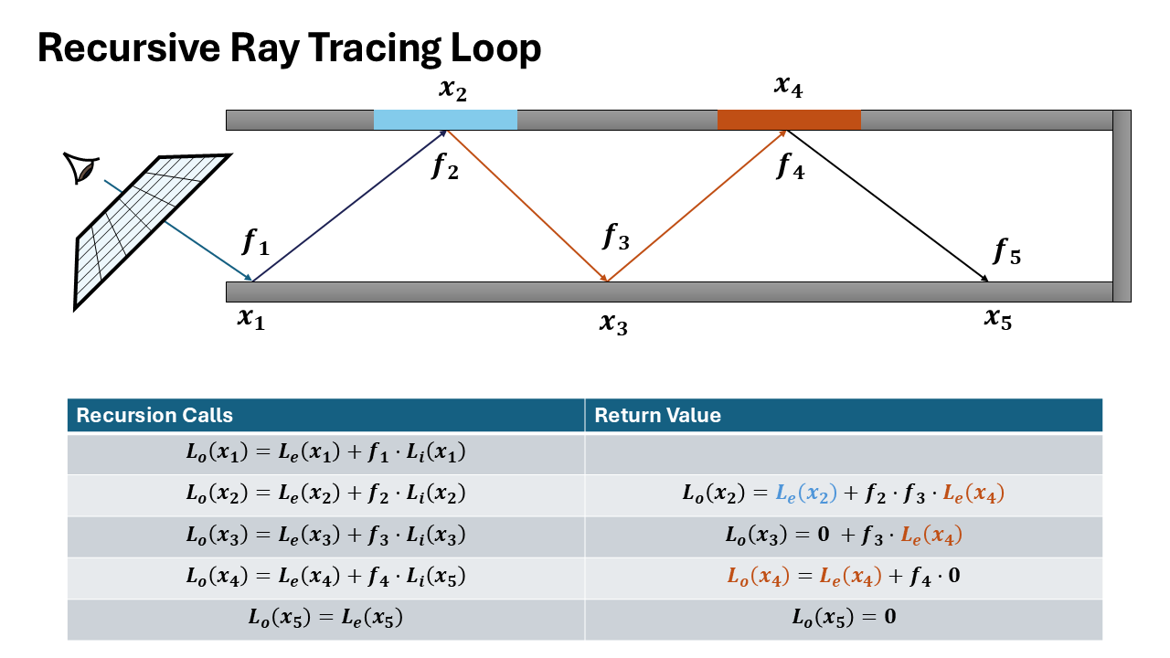
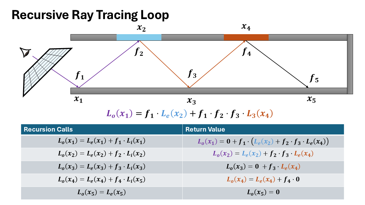
Recursion relation:
$$L_o^{(d)}(x, \omega_o) = L_e(x, \omega_o) + \frac{f_r(x, \omega_i, \omega_o) \cdot L_i^{(d+1)}(x, \omega_i)}{p(\omega_i)}$$Loop Formulation
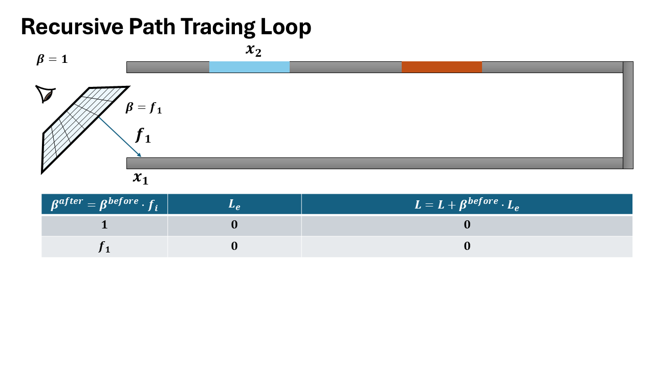
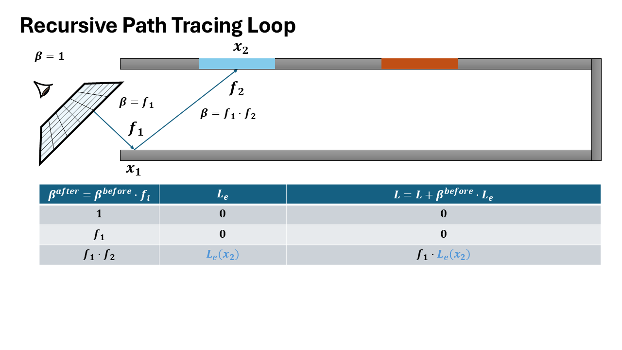
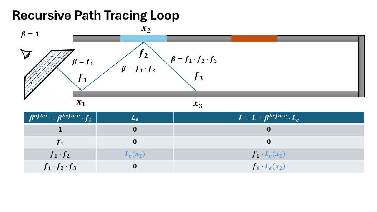
A corresponding loop version of the Path Tracing which is better for CUDA is as follows:
function PATHTRACE(scene, ray):
    depth ← 0
    f ← 1                # throughput (path weight)
    L ← 0                # accumulated radiance

    while depth < max_depth
        si ← INTERSECT(ray, scene)
        if not si.valid():
            break

        bsdf ← si.bsdf()
        Lₑ ← si.emission()
        L ← L + f * Lₑ   # accumulate emitted radiance

        (ωᵢ, fᵣ, pᵢ) ← BSDF_SAMPLE(bsdf)
        if pᵢ == 0:
            break

        f ← f * (fᵣ / pᵢ)   # update throughput
        ray ← RAY(si.p, ωᵢ)

        # Russian roulette termination
        if depth ≥ rr_depth:
            q ← max(f.x, f.y, f.z)
            if RAND() > q:
                break
            f ← f / q

        depth ← depth + 1

    return L
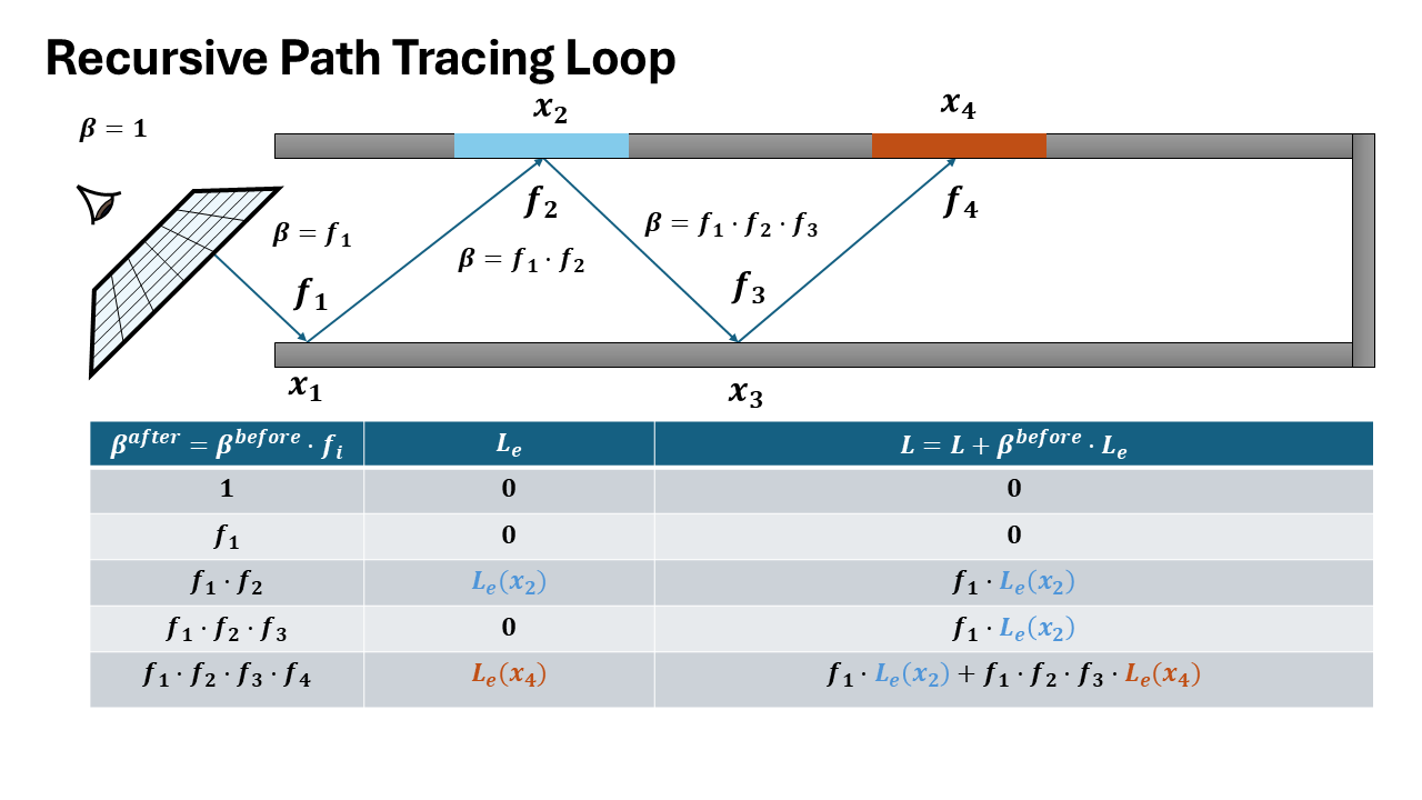
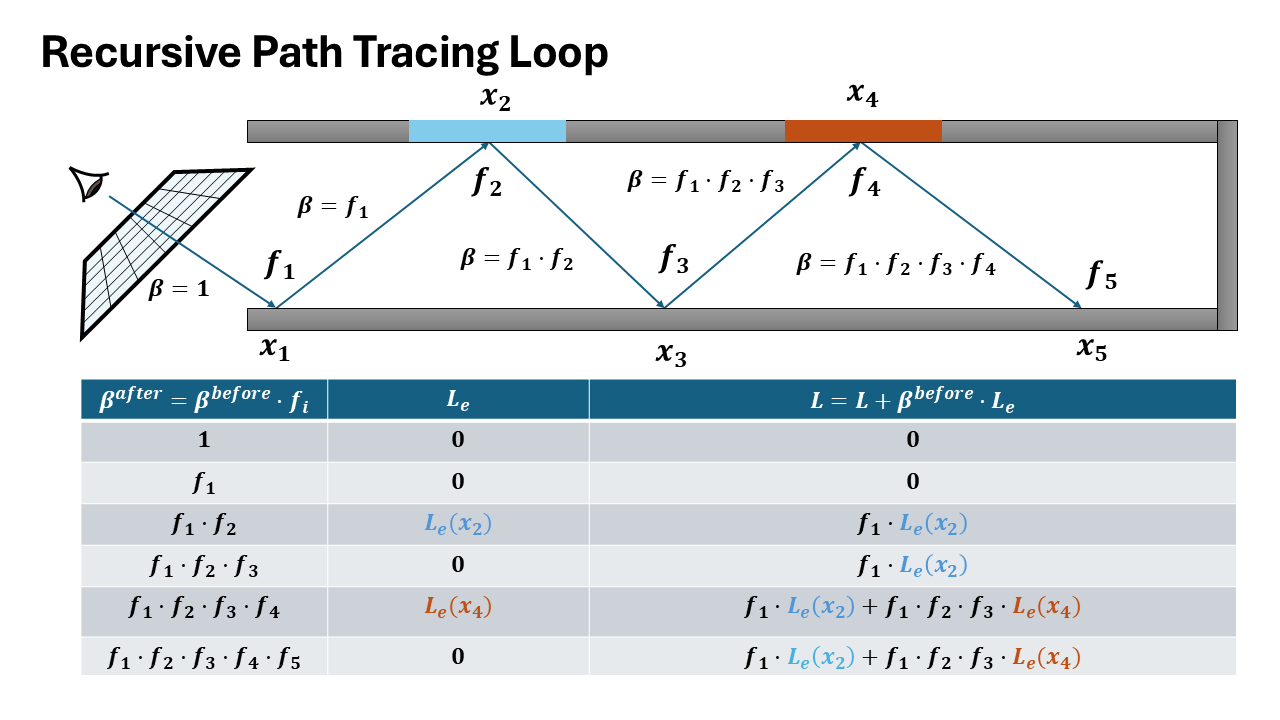
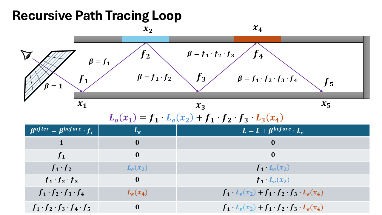
Accumulation relation:
$$L = \sum_{d=0}^{\infty} f^{(d)} \cdot L_e^{(d)}$$where $f^{(d)} = \prod_{k=0}^{d-1} \frac{f_r^{(k)}}{p_i^{(k)}}$
Equivalence
Both formulations are mathematically equivalent. The recursive form (Alg. 1) naturally expresses the rendering equation recursion, while the iterative form (Alg. 2) is more efficient for GPU implementation:
- Recursive: Computes $L_o$ by solving the implicit equation directly
- Iterative: Unrolls the recursion, accumulating contributions at each bounce with throughput $f$
The loop version materializes the infinite recursion by:
- Maintaining throughput $f$ instead of computing implicit weights
- Accumulating $L_e$ contributions at each step (line 14)
- Early termination via Russian roulette when $f \approx 0$
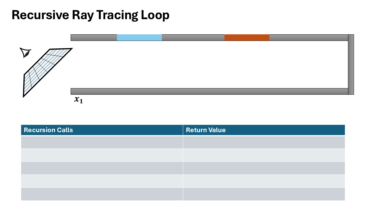
Visualization of both recursive and iterative formulation


How it matters for data collection
The recursive formulation provides direct access to intermediate incoming radiance values at each intersection point along the path. When recursively tracing a ray, at each bounce depth $d$, you immediately have:
- $L_i^{(d)}$: incoming radiance at intersection $d$
- $\omega_i^{(d)}$: sampled direction at intersection $d$
- $x^{(d)}$: surface position and properties
In contrast, the iterative formulation only accumulates the final radiance over the entire path, computing a single value $L$ by threading throughput forward. The incoming radiance at intermediate intersections is never explicitly computed or stored.
To extract per-bounce training data from the iterative formulation, you must perform a backward pass to decompose the accumulated radiance back to each path vertex-an expensive additional computation step.
Path Tracing Integrator in Mitsuba
Mitsuba 3 is a research-oriented retargetable rendering system, written in portable C++17 on top of the Dr.Jit Just-In-Time compiler.
I am going to use the python bindings of Mitsuba and it’s components to show how a standard Path Tracer works. First we need to set up all the objects as given in the Assumptions.
First the Sensor/Camera generates the initial rays that we are going to trace.
class PinholeSensor(mi.Sensor):
    def __init__(self, props):
        super().__init__(props)
        self.m_fov = props.get('fov', 45.0)
        self.m_film = props.get('film')
        self.m_sampler = props.get('sampler')
        self.m_to_world = props.get('to_world', mi.ScalarTransform4f())

    def sample_ray(self, time, sample1, sample2, active=True):
        # Convert sample to pixel, then to ray direction
        film_size = self.film().size()
        aspect = film_size[0] / film_size[1]

        # Normalized device coordinates
        ndc = (sample1 * 2.0 - 1.0) * mi.ScalarVector2f(aspect, 1.0)

        # Camera space direction
        tan_fov = dr.tan(dr.deg2rad(self.m_fov) * 0.5)
        direction = mi.ScalarVector3f(ndc.x * tan_fov,  ndc.y * tan_fov, -1.0)

        # Transform to world space
        ray = self.m_to_world @ mi.Ray3f(o=[0,0,0], d=dr.normalize(direction))
        return ray, mi.Color3f(1.0)

    def film(self): return self.m_film
    def sampler(self): return self.m_sampler

mi.register_sensor("pinhole", lambda props: PinholeSensor(props))
Then those Rays are Given to the Integrator which then traces the rays through the scene:
class Simple(mi.SamplingIntegrator):
    def __init__(self, props=mi.Properties()):
        super().__init__(props)
        self.max_depth = props.get("max_depth") # Max Depth for Tracing
        self.rr_depth = props.get("rr_depth") # Depth After which Russina Roulette Starts

    def sample(self, scene: mi.Scene, sampler: mi.Sampler, ray_: mi.RayDifferential3f, medium: mi.Medium = None, active: bool = True):
        bsdf_ctx = mi.BSDFContext() # get the bsdf context

        ray = mi.Ray3f(ray_) # Copy the Rays given by the Sensor
        depth = mi.UInt32(0) # Initialize depth to 0
        f = mi.Spectrum(1.)  # initialize throughput to 1
        L = mi.Spectrum(0.)  # Initialize Radiance to 1

        prev_si = dr.zeros(mi.SurfaceInteraction3f)

        loop = mi.Loop(name="Path Tracing", state=lambda: (
            sampler, ray, depth, f, L, active, prev_si))

        loop.set_max_iterations(self.max_depth)

        while loop(active):
            #  Intersect Ray with the Primitive in the Scene
            si: mi.SurfaceInteraction3f = scene.ray_intersect(
                ray, ray_flags=mi.RayFlags.All, coherent=dr.eq(depth, 0))

            # Get the BSDF of the intersected Primitive
            bsdf: mi.BSDF = si.bsdf(ray)

            # Direct emission
            ds = mi.DirectionSample3f(scene, si=si, ref=prev_si)
            Le = f * ds.emitter.eval(si) # Check if the primitive Emits light
            active_next = (depth + 1 < self.max_depth) & si.is_valid()

            # BSDF Sampling
            bsdf_sample, bsdf_val = bsdf.sample(
                bsdf_ctx, si, sampler.next_1d(), sampler.next_2d(), active_next)

            # Update loop variables
            ray = si.spawn_ray(si.to_world(bsdf_sample.wo))
            L = (L + Le)
            f *= bsdf_val

            prev_si = dr.detach(si, True)

            # Stopping criterion (russian roulettte)
            active_next &= dr.neq(dr.max(f), 0)

            rr_prop = dr.maximum(f.x, dr.maximum(f.y, f.z))
            rr_prop[depth < self.rr_depth] = 1.
            f *= dr.rcp(rr_prop)
            active_next &= (sampler.next_1d() < rr_prop)

            active = active_next
            depth += 1
        return (L, dr.neq(depth, 0), [])

mi.register_integrator("integrator", lambda props: Simple(props))
How to sample Next Ray Direction?
Now the above illustration was using the normalized (or approximation of normalized) BRDF Function as sampling. But there can be different ways/PDFs in which we can sample the next ray depending on the scene. A rough example is given below:
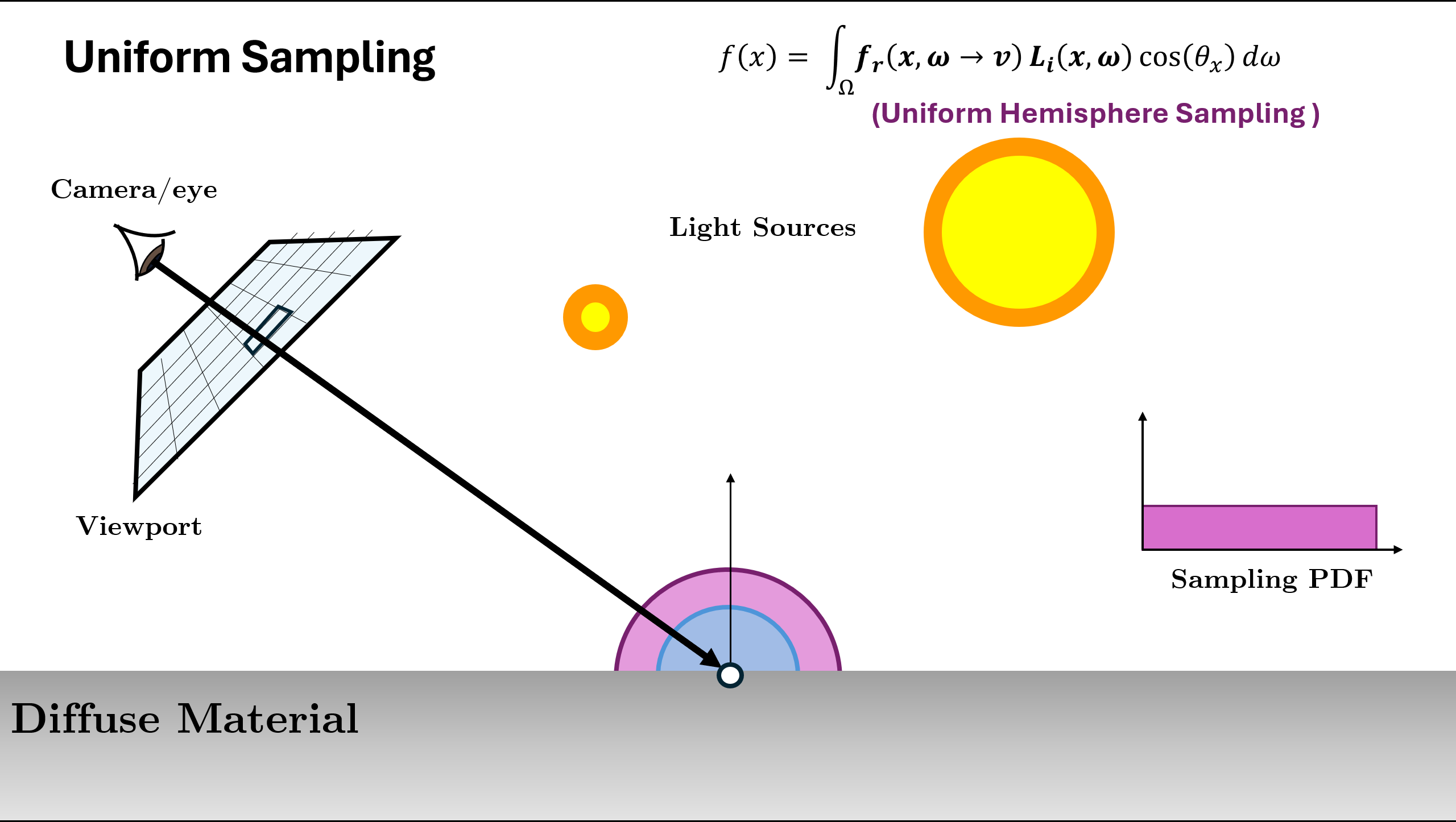
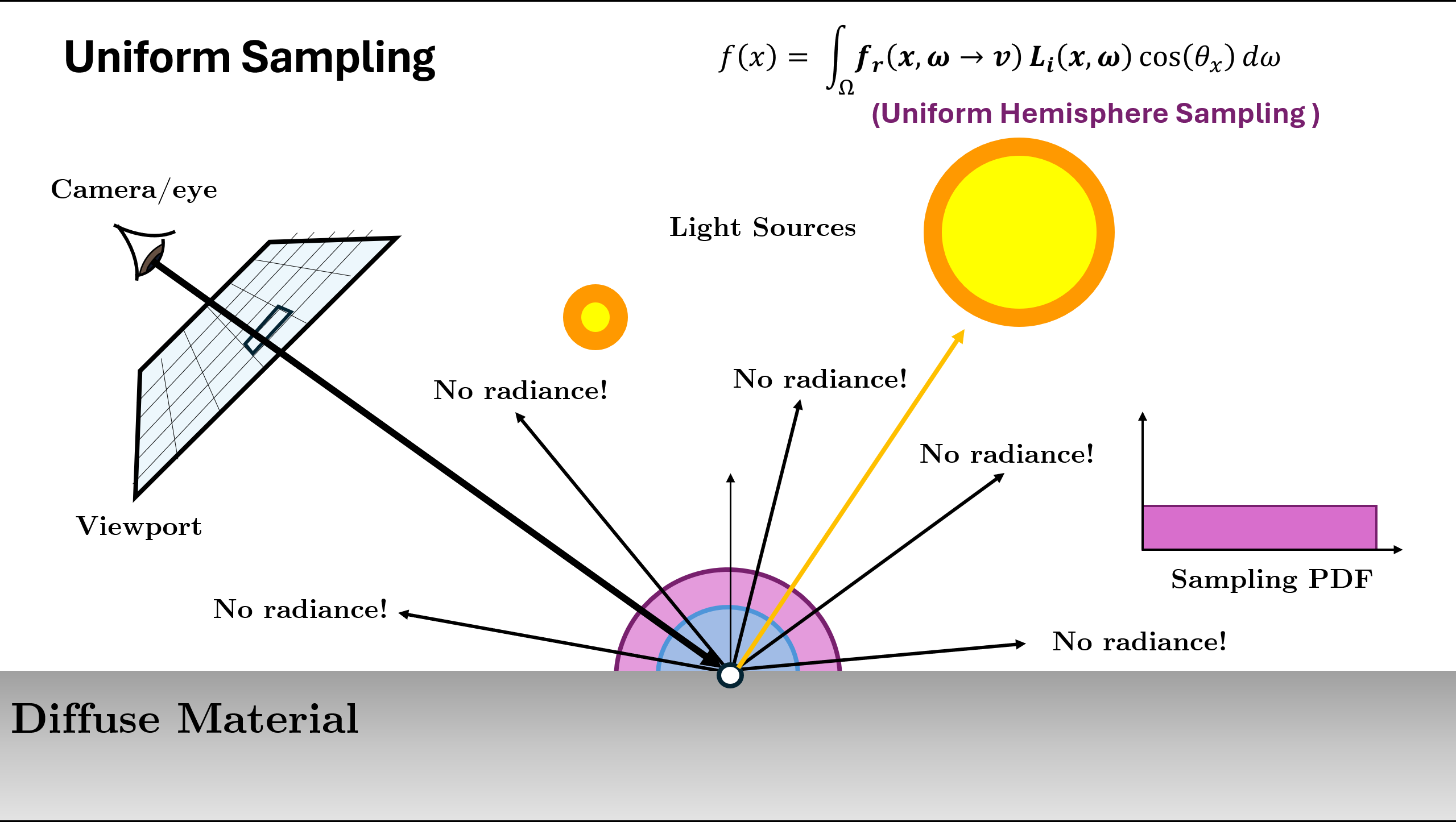

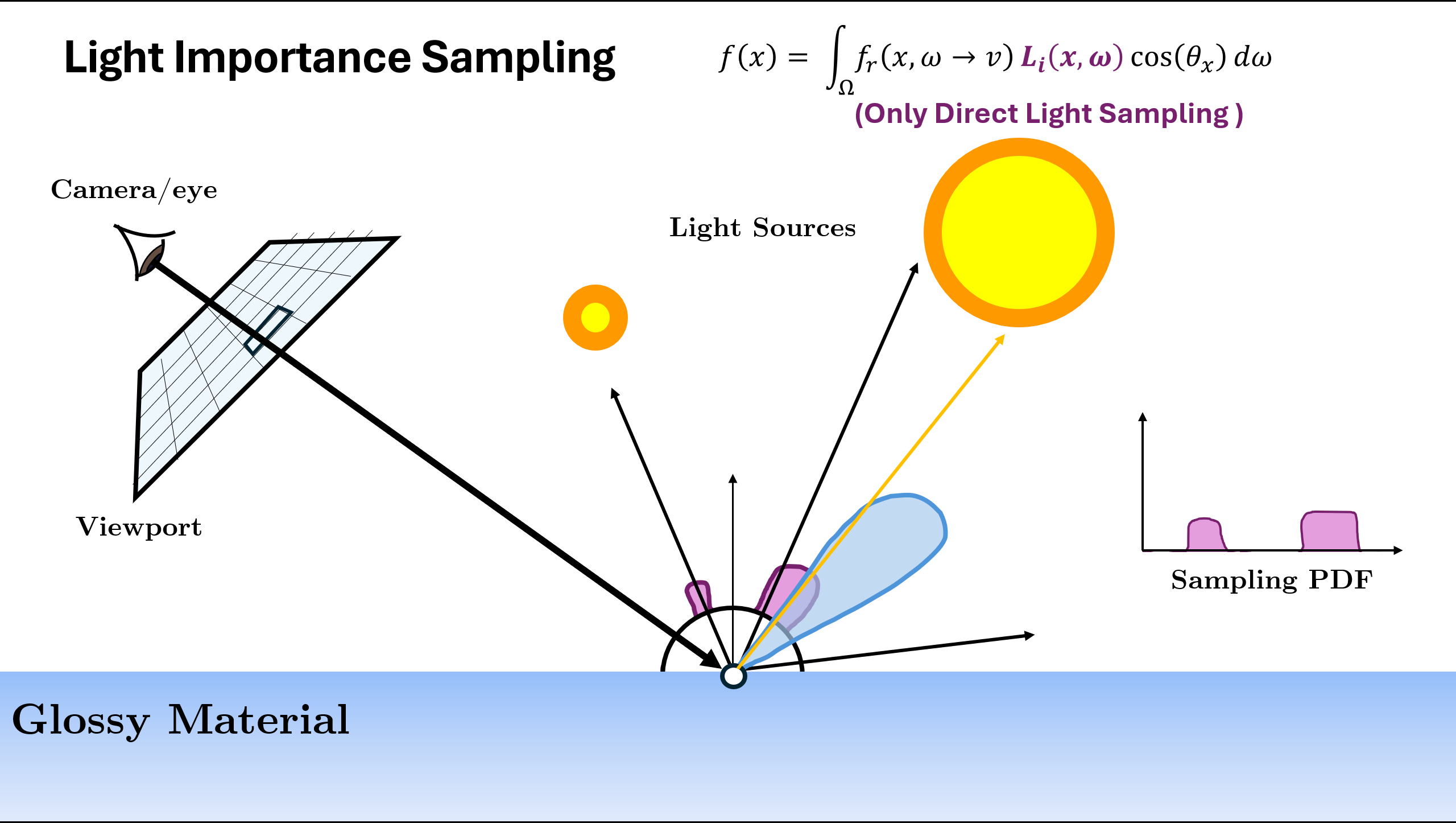
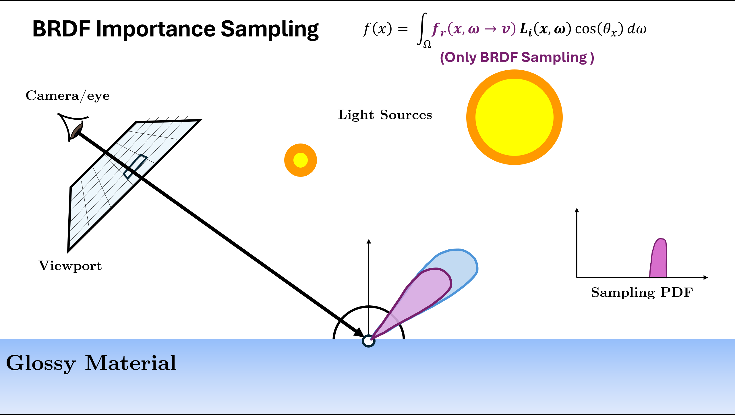
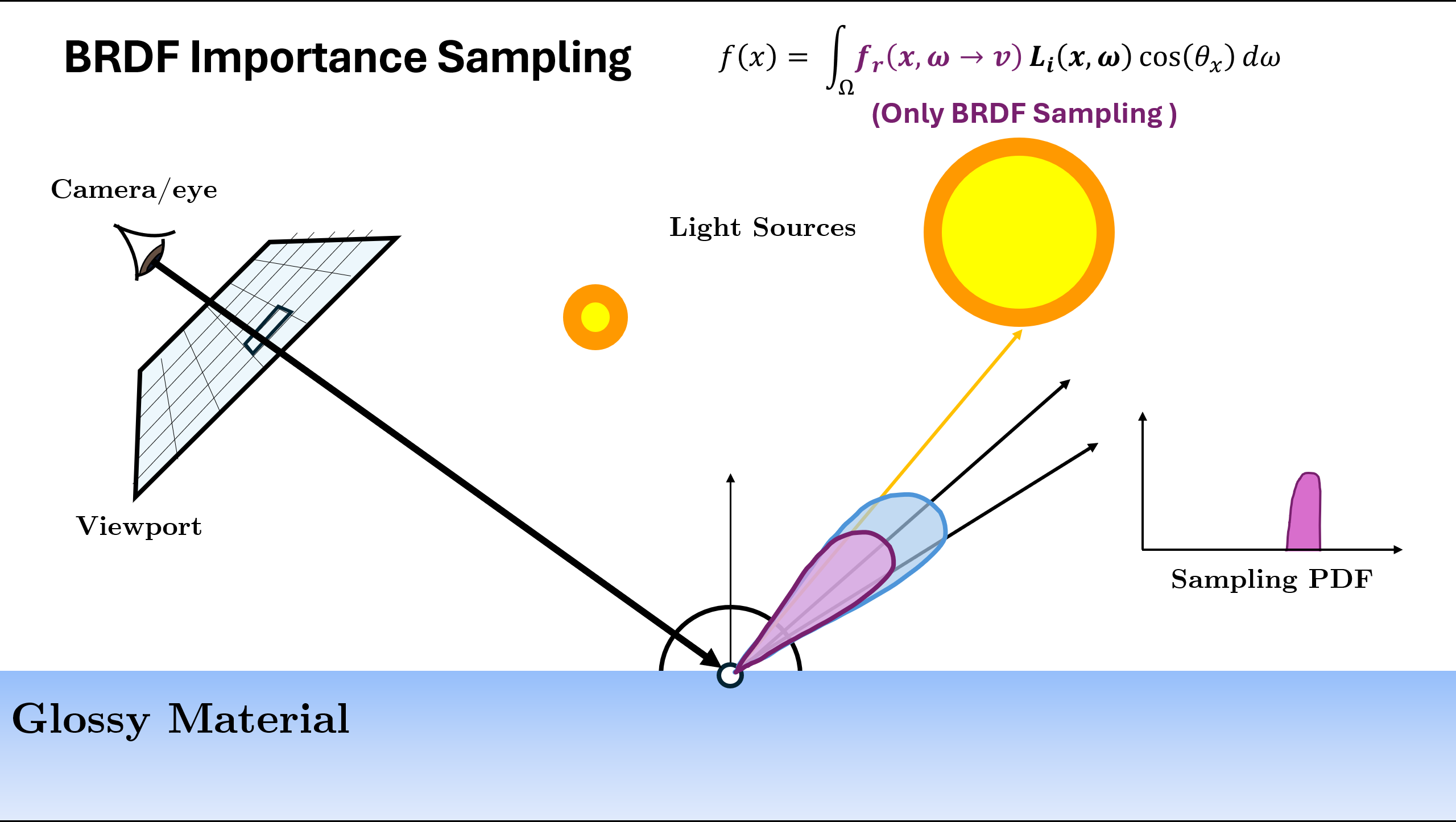
In the above example, we see that for different scene or materials, different kind of PDF $p(x)$ are better choice. The two used in above are
Now we can use these different sampling strategies, but the problem is for some parts of the scene one strategy is better whereas for other parts, the other strategy could be better. In case of the multiple sampling strategies, what to do?
Examples using a pair of scenes
I have used some renders from this amazing blog on Multiple Importance Sampling by Nikita Lisitsa.
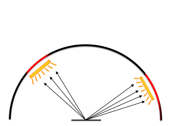
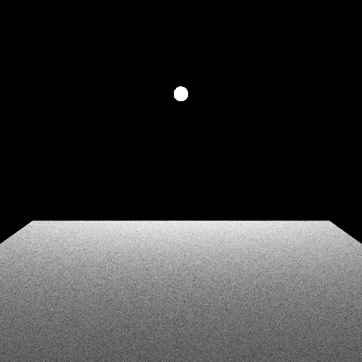
Pair of scenes: one (one the left) with a diffuse plane and a small light source, another (on the right) with a metallic plane and a large light source. One simple choice that works for diffuse materials (such that $r=const$ is to ignore the $L_{in}$ part and use a distribution proportional to the dot product $(\omega_{in}\cdot n)$) both rendered with 64 spp and uniform sampling as well as cosine weighted sampling:
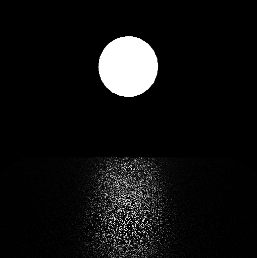
However, it doesn’t help much with the above scenes neither with the diffuse plane nor with the metallic surface. In these cases, both the uniform distribution and the cosine-weighted one poorly approximate the integrated function
- For the diffuse surface, they are good approximations of the BRDF term, but they poorly approximate the incoming light since the light comes only from a handful of directions pointing to the small sphere
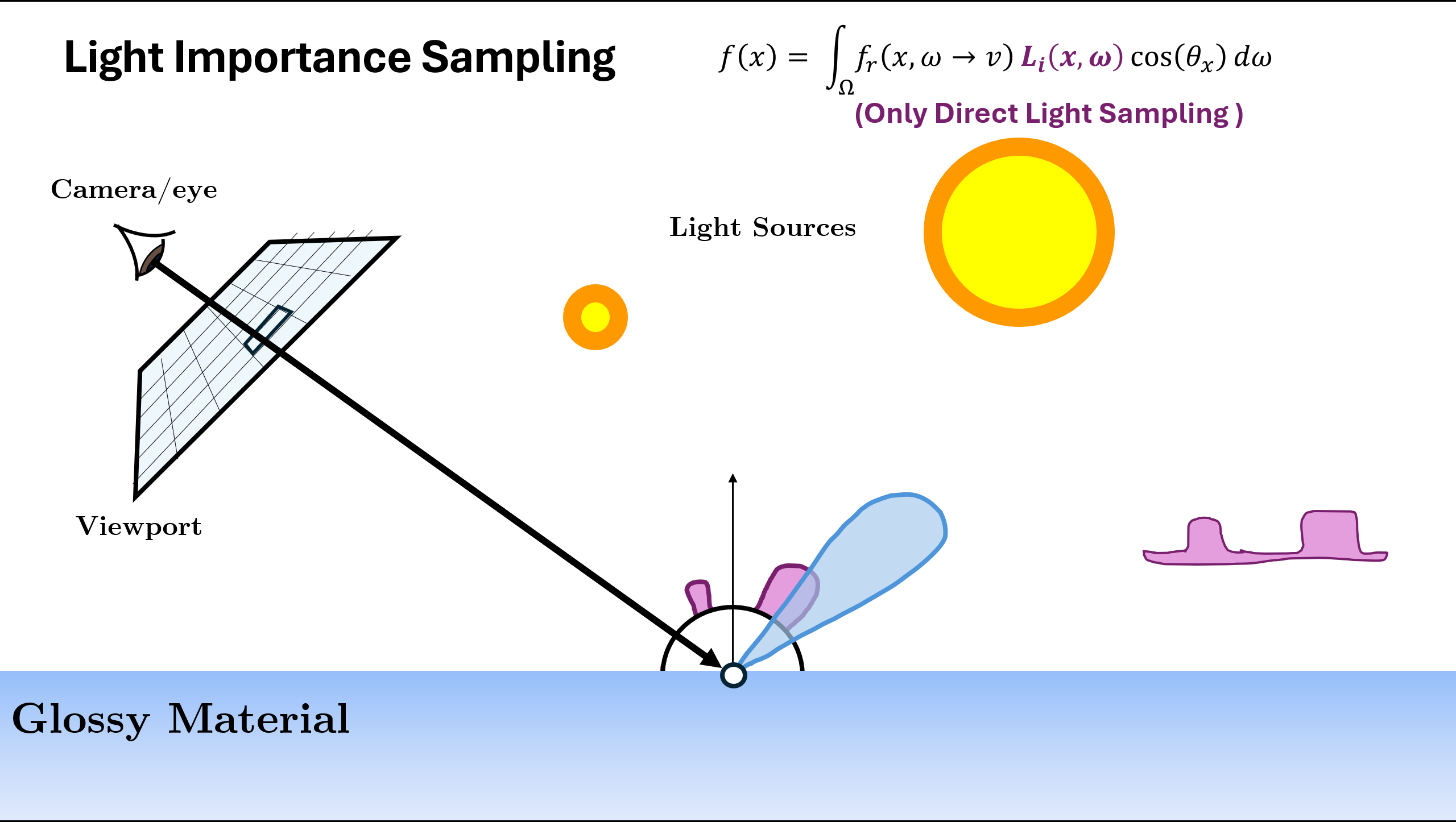
- For the metallic surface, they are OK approximations of the incoming light (which now comes from a lot of directions, because the light source is quite big), but they are poor approximations of the BRDF term, which for nice polished metals wants to reflect light only in a certain direction, and not in a random one
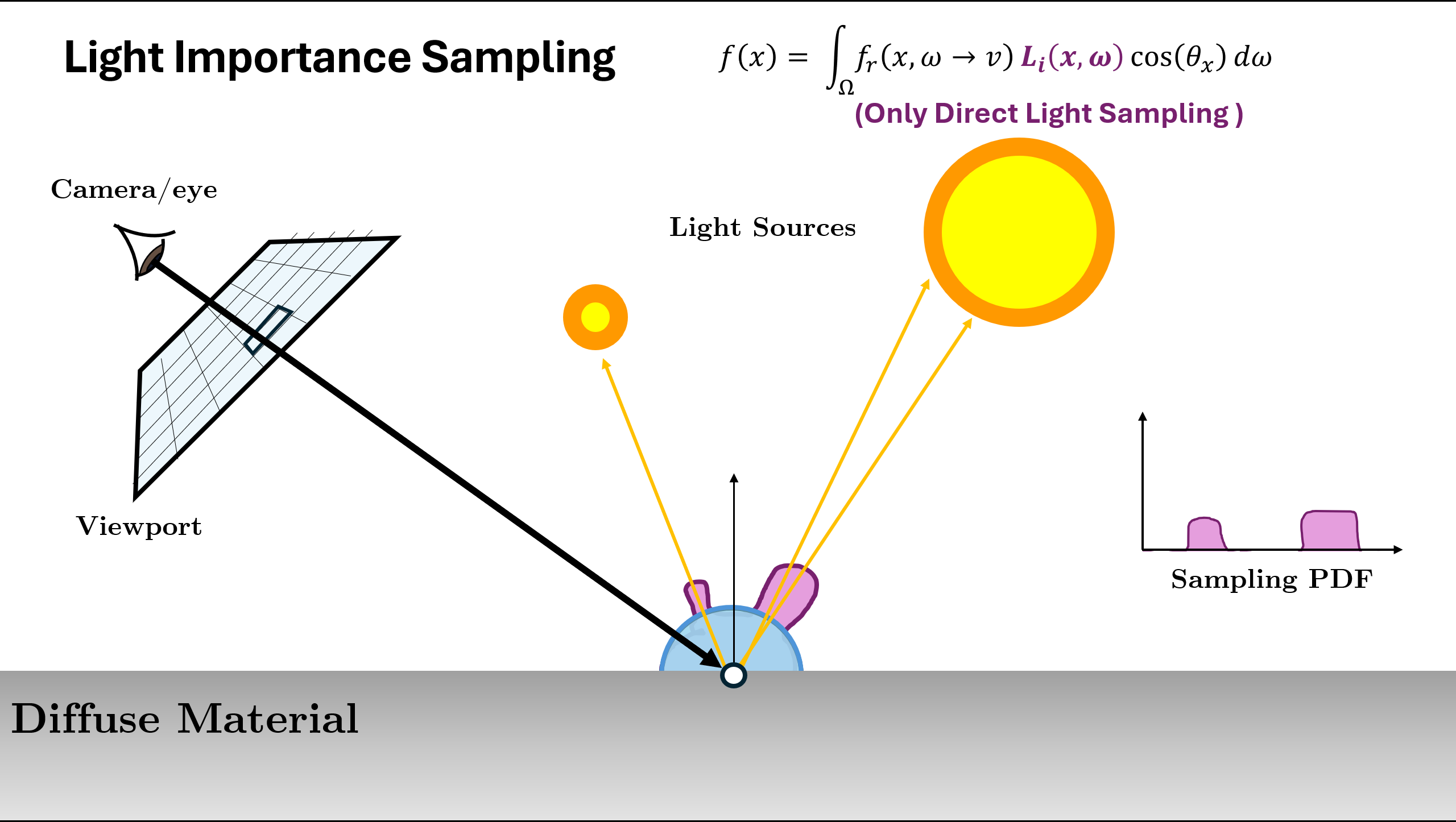
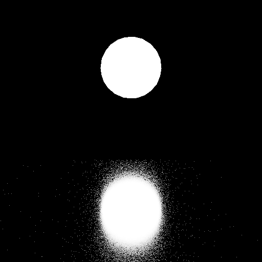
Thus, we can use the following sampling strategies for the scenes respectively:
- Send random directions directly to the light source! This is called direct light sampling, or light importance sampling, or just light sampling
- One thing we can do for the metallic plane is to figure out a distribution that sends more rays towards the direction of perfect reflection. This distribution is called VNDF
Product Function Integral
We are frequently face with integrals that are product of two or more functions: $\int f_a(x)f_b(x)dx$. It is often possible to derive separate sampling strategies for individual factors individually, though not one that is similar to their product. THis situation if especially common in the integrals involved with light transport, such as in the product BSDF, incident radiance and a cosine factor in the light transport equation.
To understand the challenges involved with applying Monte Carlo to such products, assume for now the good fortune of having two sampling distributions $p_a$ and $p_b that match the distributions of $f_a$ and $f_b$ exactly (In practice, this will not normally be the case). With Monte Carlo estimator, we have two options:
Sample using $p_a$, which gives estimator:
$$ \frac{f(X)}{p_a(x)} = cf_b(X) $$where $c$ is a constant equal to the integral of $f_a$, since $p_a(x) \propto f_a(x)$. The variance of this estimator is proportional to the variance of $f_b$, which may itself be high. Conversely, we might sample form $p_b$, though doing so gives us an estimator with variance proportional to the variance of $f_a$, which may similarly be high. . In the more common case where the sampling distributions only approximately match one of the factors, the situation is usually even worse.
Unfortunately, the obvious solution of taking some samples from each distribution and averaging the two estimators is not much better. Because variance is additive, once variance has crept into an estimator, we cannot eliminate it by adding it to another low-variance estimator.
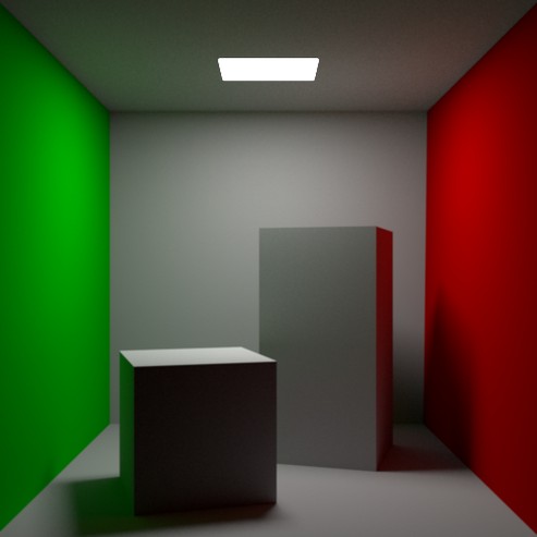
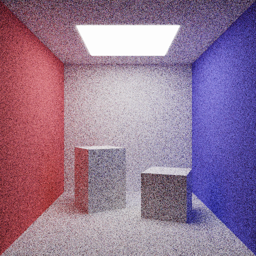
MIS Motivating Example
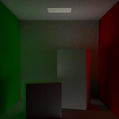
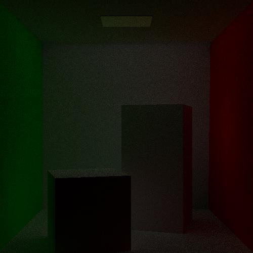
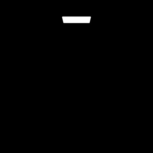
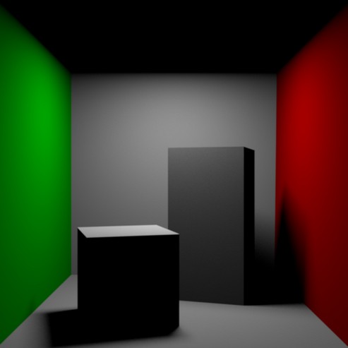
The following is a Cornell Box scene with all diffuse materials. The sampling is done in following ways
- Direct Light Sampling
- Cosine Weighted Sampling
- Direct Light Sampling
- MIS (Cosine Weighted + Direct Light Sampling)
In the Cornell box scene, we have a lot of diffuse light spreading around the scene, and using just direction light sampling produces a wrong image. The reason is that the requirement $f(x)>0 \Rightarrow p(x)>0$ is not fulfilled for this distribution: there are a lot of directions with non-zero values of our integrated function (namely, the diffuse reflections of light by the objects in the scene), but the distribution only samples a certain subset of directions (those leading directly to a light source).
So, we have a bunch of sampling strategies (i.e. a bunch of distributions), and each of them works in some cases and doesn’t work in other cases.
How can we combine several distributions at once? One obvious way would be to, say, each time we generate a sample, select one of the distributions at random and just use it in our calculations.
For example, if we have two distributions $p_1(x)$ and $p_2(x)$, we flip a fair coin, and with probability 1/2 our estimator is either $\frac{f(X)}{p_1(X)}$ or $\frac{f(X)}{p_2(X)}$. Using cosine-weighted distribution for p1, and direct light sampling for p2, we get the Wrong MIS (given below).
To get a correct combination of these pdf we have Multiple Importance Sampling
Multiple Importance Sampling (MIS)
Multiple importance sampling (MIS) addresses exactly this issue, with an easy-to-implement variance reduction technique
The basic idea is that, when estimating an integral, we should draw samples from multiple sampling distributions, chosen in the hope that at least one of them will match the shape of the integrand reasonably well, even if we do not know which one this will be. MIS then provides a method to weight the samples from each technique that can eliminate large variance spikes due to mismatches between the integrand’s value and the sampling density.
Definition - Multiple Importance Sampling
With two sampling distributions $p_a$ and $p_b$ and a single sample taken from each one, $X\sim p_a$ and $Y\sim p_b$, the MIS Monte Carlo Estimator is defined as:
$$w_a(X)\frac{f(X)}{p_a(X)} + w_b(Y)\frac{f(Y)}{p_b(Y)}$$where $w_a$ and $w_b$ are weightin functions chosen such that the expected value of this estimator is the value of integral of $f(x)$
More generally, given $n$ sampling distributions $p_i$ with $n_i$ samples $X_{i,j}$ taken from the $i$-th distribution, the MIS Monte Carlo estimator is:
$$F_n = \sum_{i=1}^{n}\frac{1}{n_i}\sum_{j=1}^{n_i}w_i(X_{i, j}) \frac{f(X_{i, j})}{p_i(X_{i, j})}$$
The full set of conditions on the weighting functions for the estimator to be unbiased are that they sum to 1 when $f(x)\neq 0$, $\sum_{i=1}^{n}w_i(x)=1$ and that $w_i(x)=0$ if $p_i(x)=0$.
In practice, a good choice for the weighting functions is given by the balance heuristic, which attempts to fulfill this goal by taking into account all the different ways that a sample could have been generated, rather than just the particular one that was used to do so. The balance heuristic’s weighting function for the th sampling technique is :
$$ w_i(x) = \frac{n_ip_i(x)}{\sum_j n_j p_j(x)} $$The power heuristic often reduces variance even further. For an exponent $\beta$, the power heuristic is
$$ w_i(x) = \frac{(n_ip_i(x))^\beta}{\sum_j (n_j p_j(x))^\beta} $$
Russian Roulette
Russian roulette is a technique that can improve the efficiency of Monte Carlo estimates by skipping the evaluation of samples that would make a small contribution to the final result.
Select a termination probability $q$. With probability $q$, skip evaluation and contribute $c = 0$. With probability $1-q$, evaluate and weight by $\frac{1}{1-q}$:
$$ \boxed{ \hat{I}_{RR} = \begin{cases} 0 & \text{with probability } q \\ \frac{\hat{I}_{MC}}{1-q} & \text{with probability } 1-q \end{cases} } $$Unbiasedness
$$ \mathbb{E}[\hat{I}_{RR}] = q \cdot 0 + (1-q) \cdot \frac{1}{1-q} \mathbb{E}[\hat{I}_{MC}] = \mathbb{E}[\hat{I}_{MC}] = I $$The estimator remains unbiased despite skipping samples.
With these Monte Carlo foundations in place, let’s examine how path tracing implements these concepts in practice.
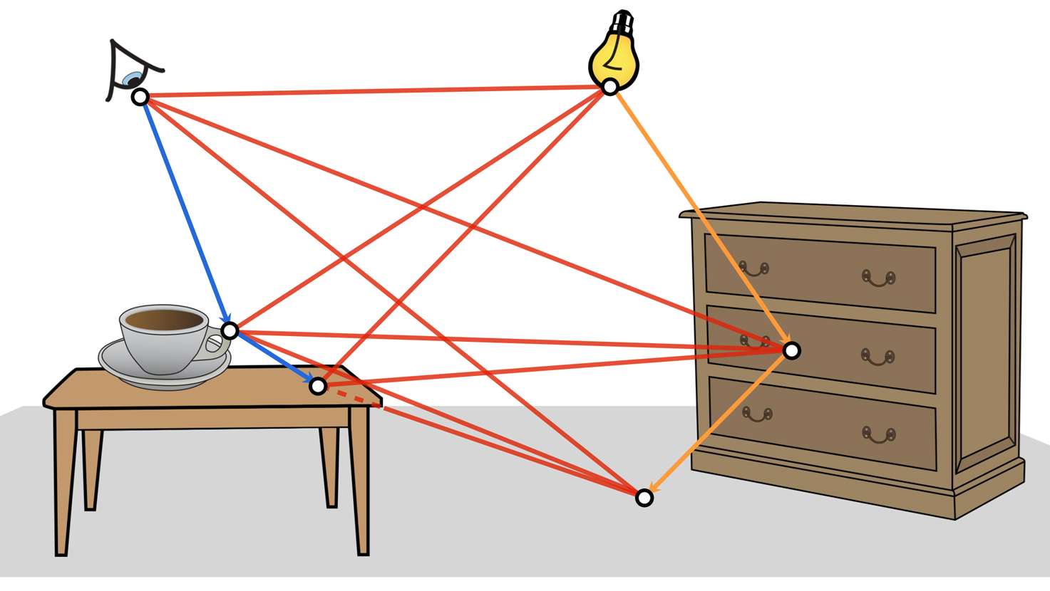
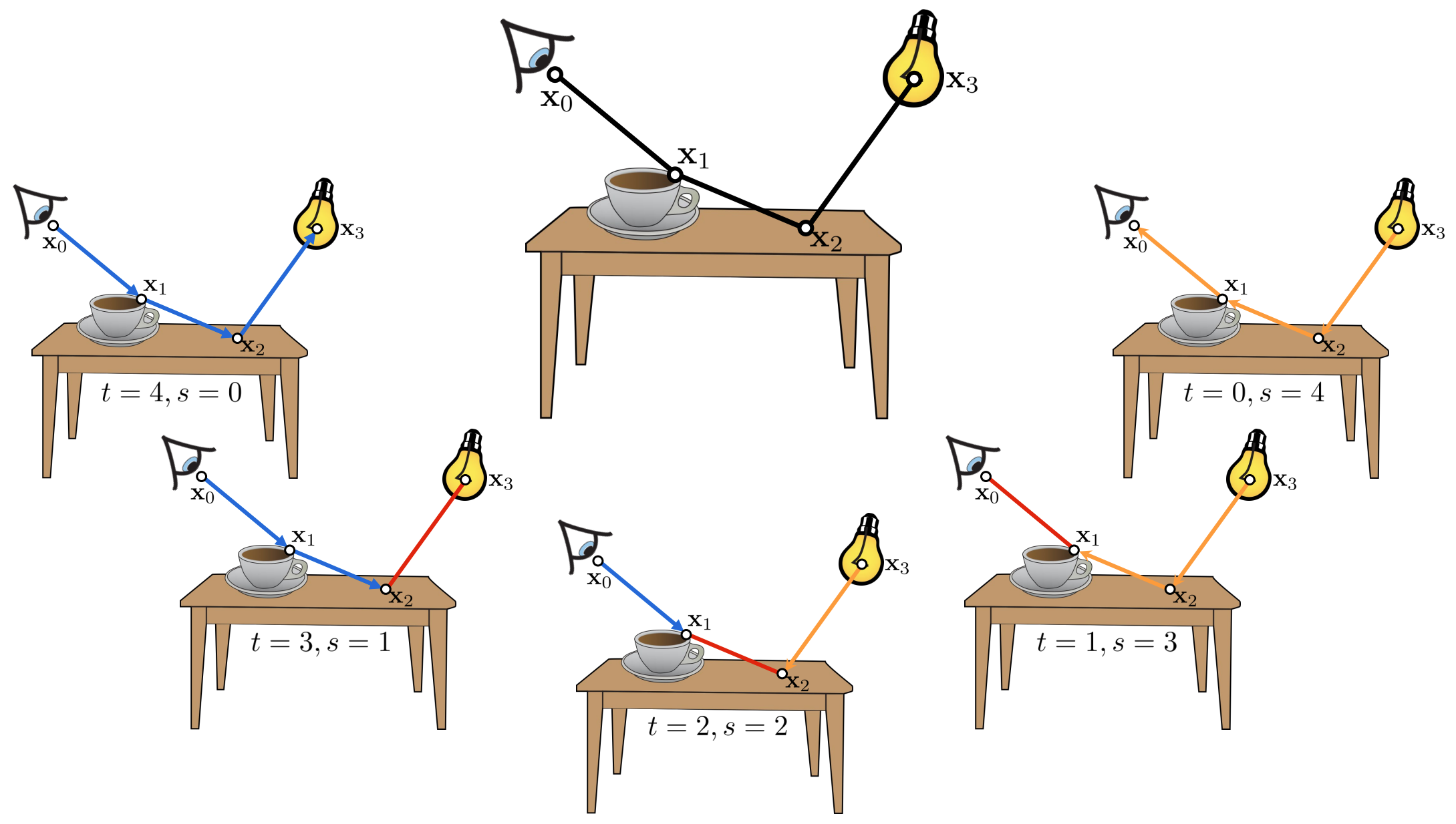
Combining multiple Paths
We now have looked at different methods of combining different samples. We can now look at the path integral formulation and look at individual path sinstead of the next direction. We can observe that we can construct paths using multiple techniques and also combine all of them as visualized below. I’ve used the images from the CMU 15-468: Physically Based Rendering and Advanced Image Synthesis course webpage and can be referred for more details.
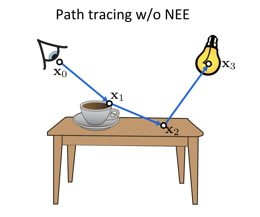
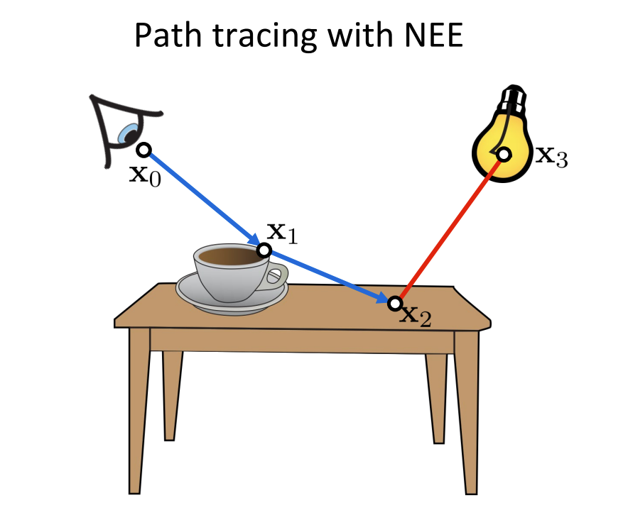
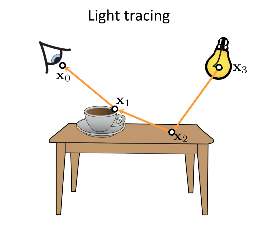
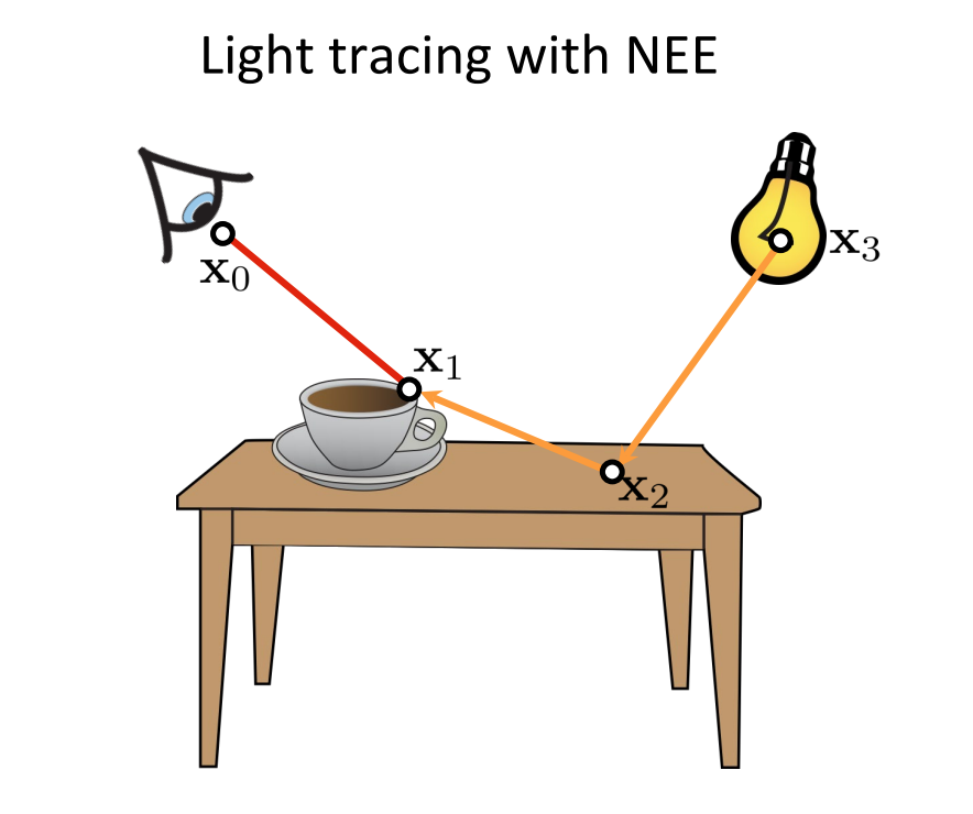
We have seen how individual paths are constructed using different techniques, we can combine all of them (using NEE at every vertex) and construct many paths using only a few vertices.
| Symbol | Meaning |
|---|---|
| $t$ | Number of vertices on camera subpath |
| $s$ | Number of vertices on light subpath |
| $ts$ | Number of connections |
A look at the Importance Sampling Techniques
Overview
The techniques we’ve covered (importance sampling, MIS, Russian roulette) all rely on choosing good sampling distributions. We used some examples like (BRDF, Direct Light Sampling, VNDF) but now we will take a look at some methods which try to learn these distributions using the samples generated during rendering.
Neural methods learn these distributions from data, enabling near-optimal importance sampling in complex scenes. The papers below represent the evolution of this idea of choosing/designing $p(x)$ carefully.
| Paper | Venue |
|---|---|
| Path Guiding Using Spatio-Directional Mixture Models | EGSR (2014) |
| Practical Path Guiding for Efficient Light-Transport Simulation | EGSR (2017) |
| Offline Deep Importance Sampling | Pacific Graphics (2018) |
| Neural Importance Sampling | SIGGRAPH (2019) |
| Real-time Neural Radiance Caching for Path Tracing | SIGGRAPH (2021) |
| Neural Parametric Mixtures for Path Guiding | SIGGRAPH (2023) |
| Online Neural Path Guiding with Normalized Anisotropic Spherical Gaussians | ACM TOG (2024) |
| Neural Product Importance Sampling via Warp Composition | SIGGRAPH Asia (2024) |
| Neural Path Guiding with Distribution Factorization | EGSR (2025) |
While a lot more methods have emerged (not necessarily neural), I will add them once I read them in detail and the above papers are what I feel cover a good amount of methods over the years from foundational to recent methods.
Neural Importance Sampling
Overview
Neural Importance Sampling (NIS) proposes to use deep neural networks for generating samples in Monte Carlo integration . The approach is based on Non-linear Independent Components Estimation (NICE), extended with novel coupling transforms and optimization strategies specifically designed for integration problems . The key innovation is learning expressive sampling densities $q(x;\theta)$ that closely match the integrand $f(x)$, thereby reducing estimation variance .
Given an integral:
$$ F = \int_D f(x) dx $$we introduce a probability density function (PDF) $q(x)$ to express $F$ as an expected ratio :
$$ F = \int_D \frac{f(x)}{q(x)} q(x) dx = \mathbb{E}\left[\frac{f(X)}{q(X)}\right] $$This expectation can be approximated using $N$ independent samples $\{X_1, X_2, \ldots, X_N\}$ where $X_i \in D, X_i \sim q(x)$ :
$$ F \approx \langle F \rangle_N = \frac{1}{N} \sum_{i=1}^{N} \frac{f(X_i)}{q(X_i)} $$The variance of this estimator heavily depends on how closely $q$ matches the normalized integrand $p(x) \equiv f(x)/F$ . In the ideal case where samples are drawn from a PDF proportional to $f(x)$, we obtain a zero-variance estimator .
Normalizing Flows and NICE
Neural Importance Sampling leverages normalizing flows to model the sampling distribution as a deterministic bijective mapping $x = h(z;\theta)$ from a simple latent distribution $q(z)$ (e.g., uniform or Gaussian) to the complex target distribution . The probability density is computed using the change-of-variables formula:
$$ q(x;\theta) = q(z) \left|\det\left(\frac{\partial h(z;\theta)}{\partial z^T}\right)\right|^{-1} $$where the inverse Jacobian determinant accounts for density changes due to the transformation .
For this to be practical in Monte Carlo integration, three requirements must be satisfied :
- Tractable inverse: Given $x$, we must efficiently compute $z = h^{-1}(x)$
- Fast evaluation: Both $h$ and $h^{-1}$ must be computationally efficient
- Tractable Jacobian: The Jacobian determinant must be efficiently computable
NICE satisfies all these requirements through coupling layers that admit triangular Jacobian matrices with determinants reducing to products of diagonal terms .
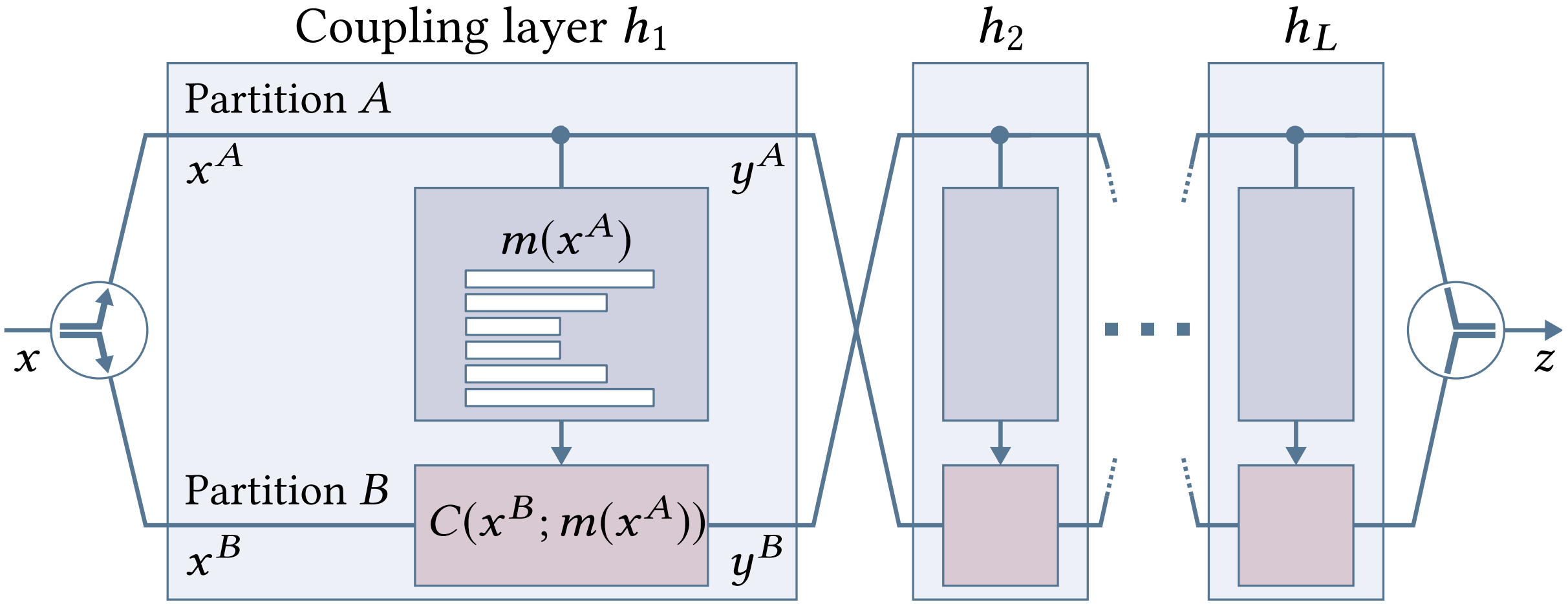
Coupling Layers
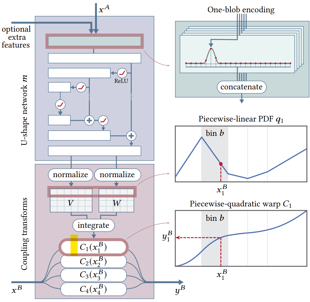
A coupling layer partitions the $D$-dimensional input vector $x$ into two disjoint groups $A$ and $B$ . It leaves partition $A$ unchanged while using it to parameterize the transformation of partition $B$:
$$ y_A = x_A $$$$ y_B = C(x_B; m(x_A)) $$where $C: \mathbb{R}^{|B|} \times m(\mathbb{R}^{|A|}) \to \mathbb{R}^{|B|}$ is a separable and invertible coupling transform, and $m$ is a neural network .
The invertibility is trivial :
$$ x_A = y_A $$$$ x_B = C^{-1}(y_B; m(x_A)) = C^{-1}(y_B; m(y_A)) $$Since $C$ is separable by design, its Jacobian matrix is diagonal, making determinant computation tractable even in high dimensions . The complete transformation is obtained by compounding multiple coupling layers $\tilde{h} = h_L \circ \cdots \circ h_2 \circ h_1$, alternating which partition is transformed .
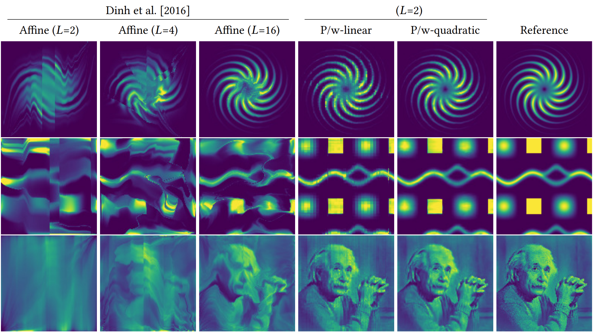
Piecewise-Polynomial Coupling Transforms
Instead of the affine (multiply-add) coupling transforms from prior work, Neural Importance Sampling introduces piecewise-polynomial coupling transforms with significantly greater modeling power .
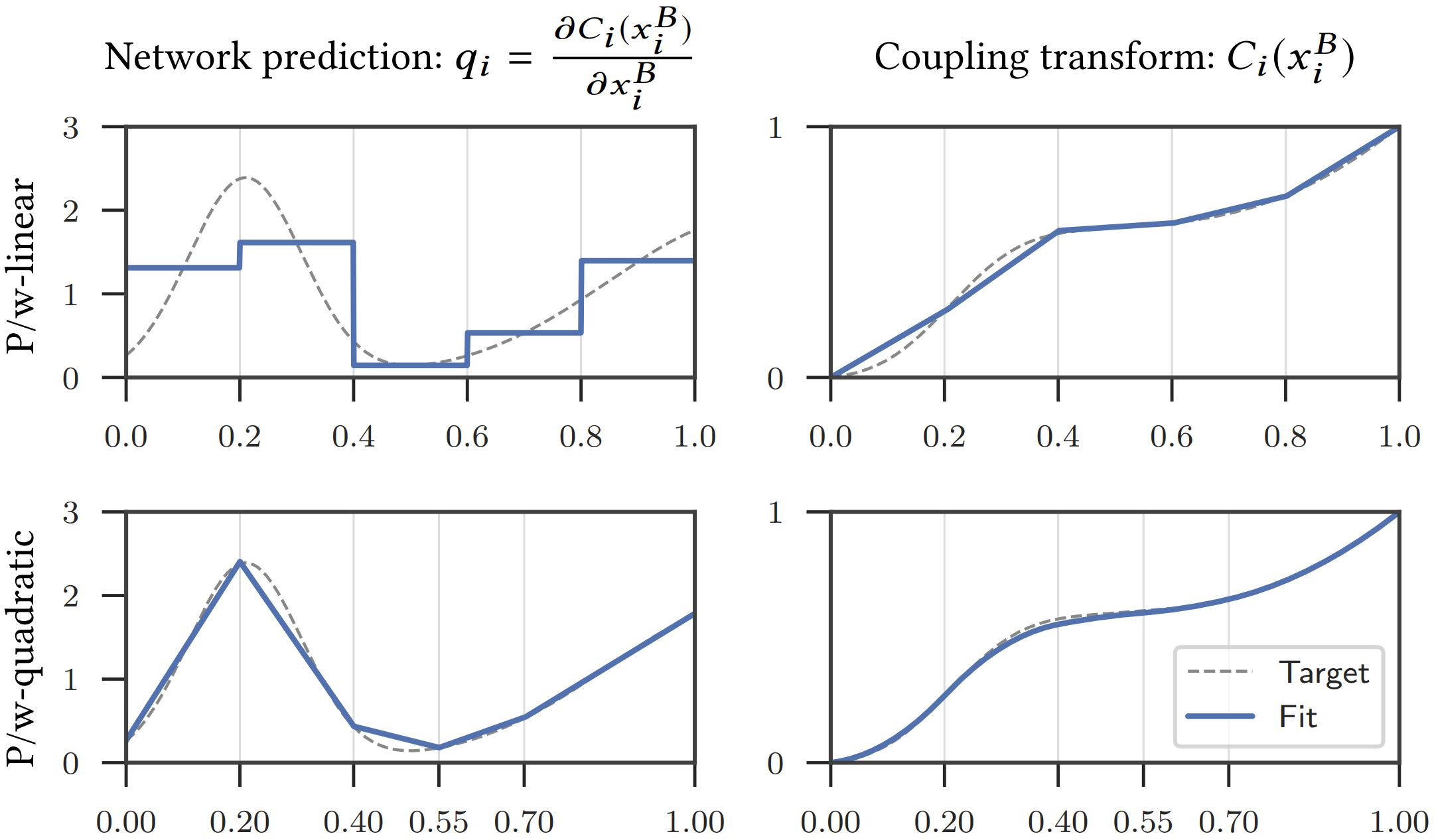
Piecewise-Linear Coupling Transform
The approach operates on the unit hypercube $x, y \in [0,1]^D$ with uniformly distributed latent variables . Each dimension in partition $B$ is divided into $K$ bins of equal width $w = 1/K$ .
The neural network $m(x_A)$ outputs a $|B| \times K$ matrix $\tilde{Q}$, where each row defines an unnormalized probability mass function . After softmax normalization $Q_i = \sigma(\tilde{Q}_i)$, the PDF in dimension $i$ is:
$$ q_i(x_i^B) = \frac{Q_{ib}}{w} $$where $b = \lfloor Kx_i^B \rfloor$ is the bin containing $x_i^B$ .
The piecewise-linear coupling transform is obtained by integration :
$$ C_i(x_i^B; Q) = \int_0^{x_i^B} q_i(t) dt = \alpha Q_{ib} + \sum_{k=1}^{b-1} Q_{ik} $$where $\alpha = Kx_i^B - \lfloor Kx_i^B \rfloor$ represents the relative position within bin $b$ .
The Jacobian determinant reduces to :
$$ \det\left(\frac{\partial C(x^B; Q)}{\partial (x^B)^T}\right) = \prod_{i=1}^{|B|} q_i(x_i^B) = \prod_{i=1}^{|B|} \frac{Q_{ib}}{w} $$Piecewise-Quadratic Coupling Transform
For improved expressiveness and adaptive bin sizing, piecewise-quadratic transforms admit a piecewise-linear PDF modeled using $K+1$ vertices . The network outputs unnormalized matrices $\tilde{W}$ and $\tilde{V}$, which are normalized as:
$$ W_i = \sigma(\tilde{W}_i) $$$$ V_{i,j} = \frac{\exp(\tilde{V}_{i,j})}{\sum_{k=1}^{K} \frac{\exp(\tilde{V}_{i,k}) + \exp(\tilde{V}_{i,k+1})}{2} W_{i,k}} $$where the denominator ensures $V_i$ represents a valid PDF .
The PDF is defined as :
$$ q_i(x_i^B) = \text{lerp}(V_{ib}, V_{ib+1}, \alpha) $$where $\alpha = (x_i^B - \sum_{k=1}^{b-1} W_{ik})/W_{ib}$ represents the relative position in bin $b$ .
The invertible coupling transform is :
$$ C_i(x_i^B; W, V) = \frac{\alpha^2}{2}(V_{ib+1} - V_{ib})W_{ib} + \alpha V_{ib} W_{ib} + \sum_{k=1}^{b-1} \frac{V_{ik} + V_{ik+1}}{2} W_{ik} $$Inverting this transform involves solving a quadratic equation, which can be done efficiently and robustly .
One-Blob Encoding
To improve network performance, one-blob encoding generalizes one-hot encoding for continuous variables . For a scalar $s \in [0,1]$ and quantization into $k$ bins (typically $k=32$), a Gaussian kernel with $\sigma = 1/k$ is placed at $s$ and discretized into the bins .
Unlike one-hot encoding, one-blob encoding is lossless for continuous variables while stimulating localization of computation . This encoding effectively shuts down certain parts of the network, allowing specialization on various sub-domains .
Network Architecture
The neural network $m$ uses a U-shaped architecture with fully connected layers . For each coupling layer:
- Input: One-blob encoded partition $A$ dimensions and optional features (position, normal, etc.)
- Architecture: Typically 8-10 fully connected layers with ReLU activations
- Outermost layers: 256 neurons, halved at each nesting level
- Output layer: Produces parameters for coupling transform ($Q$, or $W$ and $V$)
All inputs are one-blob encoded with $k=32$ bins . For 3D positions, each coordinate is normalized by the scene bounding box, encoded independently, and concatenated into a $3 \times k$ array . Directions are parameterized using cylindrical coordinates, transformed to $[0,1]$, and similarly encoded .
Optimization for Monte Carlo Integration
Minimizing KL Divergence
The Kullback-Leibler divergence between the ideal distribution $p(x)$ and learned $q(x;\theta)$ is :
$$ D_{KL}(p \| q; \theta) = \int_{\Omega} p(x) \log \frac{p(x)}{q(x;\theta)} dx $$The gradient with respect to trainable parameters $\theta$ is :
$$ \nabla_{\theta} D_{KL}(p \| q; \theta) = \mathbb{E}\left[-\frac{p(X)}{q(X;\theta)} \nabla_{\theta} \log q(X;\theta)\right] $$where the expectation is over $X \sim q(x;\theta)$ .
Since $p(x) = f(x)/F$ and $F$ is unknown, the stochastic gradient uses unnormalized estimates :
$$ \nabla_{\theta} D_{KL}(p \| q; \theta) \approx -\frac{1}{N} \sum_{j=1}^{N} \frac{f(X_j)}{q(X_j;\theta)} \nabla_{\theta} \log q(X_j;\theta) $$where $X_j \sim q(x;\theta)$ .
Minimizing Variance (χ² Divergence)
Directly minimizing the estimator variance is equivalent to minimizing the Pearson χ² divergence :
$$ \mathbb{V}\left[\frac{p(X)}{q(X;\theta)}\right] = \mathbb{E}\left[\frac{p(X)^2}{q(X;\theta)^2}\right] - \mathbb{E}\left[\frac{p(X)}{q(X;\theta)}\right]^2 $$The stochastic gradient for variance minimization is :
$$ \nabla_{\theta} \mathbb{V}\left[\frac{p(X)}{q(X;\theta)}\right] = \mathbb{E}\left[-\left(\frac{p(X)}{q(X;\theta)}\right)^2 \nabla_{\theta} \log q(X;\theta)\right] $$In practice, this becomes :
$$ \nabla_{\theta} \mathbb{V} \approx -\frac{1}{N} \sum_{j=1}^{N} \left(\frac{f(X_j)}{q(X_j;\theta)}\right)^2 \nabla_{\theta} \log q(X_j;\theta) $$Application to Path Guiding
For path guiding in rendering, the goal is to learn directional sampling densities $q(\omega|x,\omega_o)$ proportional to the product of incident illumination and BSDF in the rendering equation :
$$ L_o(x,\omega_o) = L_e(x,\omega_o) + \int_{\Omega} L(x,\omega) f_s(x,\omega_o,\omega) |\cos\gamma| d\omega $$The reflected radiance estimator is :
$$ \langle L_r(x,\omega_o) \rangle = \frac{1}{N} \sum_{j=1}^{N} \frac{L(x,\omega_j) f_s(x,\omega_o,\omega_j) |\cos\gamma_j|}{q(\omega_j|x,\omega_o)} $$Sampling Strategy
Since the integration domain is 2D (directional hemisphere), partitions $A$ and $B$ each contain one cylindrical coordinate dimension . To generate a sample:
- Draw random pair $u \in [0,1]^2$ from uniform distribution
- Pass through inverted coupling layers: $h_1^{-1}(\cdots h_L^{-1}(u))$
- Transform to cylindrical coordinates to obtain direction $\omega$
The neural network $m$ takes as input :
- One cylindrical coordinate from partition $A$ (one-blob encoded, $k=32$)
- Surface position $x$ (normalized, one-blob encoded per dimension, total $3k$)
- Outgoing direction $\omega_o$ (cylindrical coords, one-blob encoded, total $2k$)
- Surface normal $\mathbf{n}(x)$ (one-blob encoded)
- Optional additional features
MIS-Aware Optimization
When combining the learned distribution $q$ with existing techniques (e.g., BSDF sampling) using multiple importance sampling (MIS), the effective PDF becomes :
$$ q'(\omega) = c \cdot q(\omega) + (1-c) \cdot p_{f_s}(\omega) $$where $c$ is the selection probability . The networks are optimized with respect to $q'$ instead of $q$, minimizing $D(p \| q')$ where $D$ is either KL or χ² divergence .
Learned Selection Probabilities
An additional network $\hat{m}$ learns approximately optimal selection probability $c = \ell(\hat{m}(x,\omega_o))$, where $\ell$ is the logistic function . This network is optimized jointly with the coupling layer networks using the same architecture except for the output layer .
Training Procedure
Training occurs online during rendering in an interleaved fashion :
- Sample Generation: Draw samples using current network parameters
- Feedback: Evaluate integrand $f(x)$ at sample locations
- Gradient Computation: Compute stochastic gradient using KL or χ² loss
- Parameter Update: Update network weights using Adam optimizer
- Iteration: Repeat with updated network
The approach enables fast inference and efficient sample generation independently of integration domain dimensionality . Training converges rapidly, producing usable sampling distributions within seconds to minutes depending on scene complexity .
Real-time Neural Radiance Caching for Path Tracing
Overview
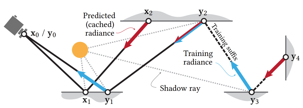
Real-time Neural Radiance Caching (NRC) is a method for accelerating path-traced global illumination by approximating the scattered radiance field using a neural network . The system handles fully dynamic scenes without assumptions about lighting, geometry, or materials . The core idea is to terminate paths early by querying a neural cache once the path spread becomes large enough to blur small inaccuracies in the cache approximation .
The neural network approximates the scattered radiance $L_s(x,\omega)$, which represents the radiative energy leaving point $x$ in direction $\omega$ after being scattered at $x$ :
$$ L_s(x,\omega) := \int_{S^2} f_s(x,\omega,\omega_i) L_i(x,\omega_i) | \cos\theta_i| d\omega_i $$where $f_s$ is the BSDF, $L_i$ is the incident radiance, and $\theta_i$ is the angle between $\omega_i$ and the surface normal at $x$ .
Algorithm Design
Rendering a single frame consists of two phases: computing pixel colors and updating the neural radiance cache .
Rendering Phase
Short rendering paths are traced (one per pixel) and terminated early when the neural cache approximation becomes sufficiently accurate . The termination criterion uses the area-spread heuristic from Bekaert et al. (2003), which compares the footprint of the path to the size of the directly visible surface in the image plane .
The area spread along subpath $x_1 \cdots x_n$ is approximated as :
$$ a(x_1 \cdots x_n) = \left(\sum_{i=2}^{n} \frac{\|x_{i-1} - x_i\|^2}{p(\omega_i \mid x_{i-1},\omega) |\cos\theta_i|}\right)^2 $$where $p$ is the BSDF sampling PDF and $\theta_i$ is the angle between $\omega_i$ and the surface normal at $x_i$ .
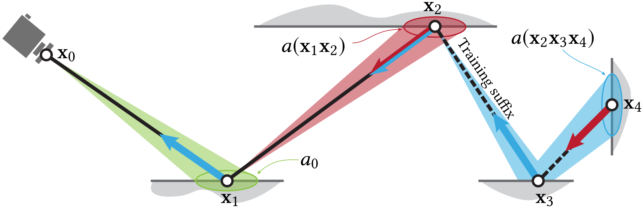
The path is terminated when $a(x_1 \cdots x_n) > c \cdot a_0$, where $c = 0.01$ is a hyperparameter and $a_0$ is the spread at the primary vertex :
$$ a_0 := \frac{\|x_0 - x_1\|^2}{4\pi \cos\theta_1} $$At the terminal vertex $x_k$, the neural radiance cache $\tilde{L}_s(x_k,\omega_k)$ is evaluated to approximate the scattered radiance .
Training Phase
A small fraction (typically under 3%) of rendering paths are extended by a few vertices to form training paths . These longer paths are terminated using the same area-spread heuristic applied to the training suffix . The collected radiance estimates along all vertices of the training paths serve as reference values for updating the neural cache .
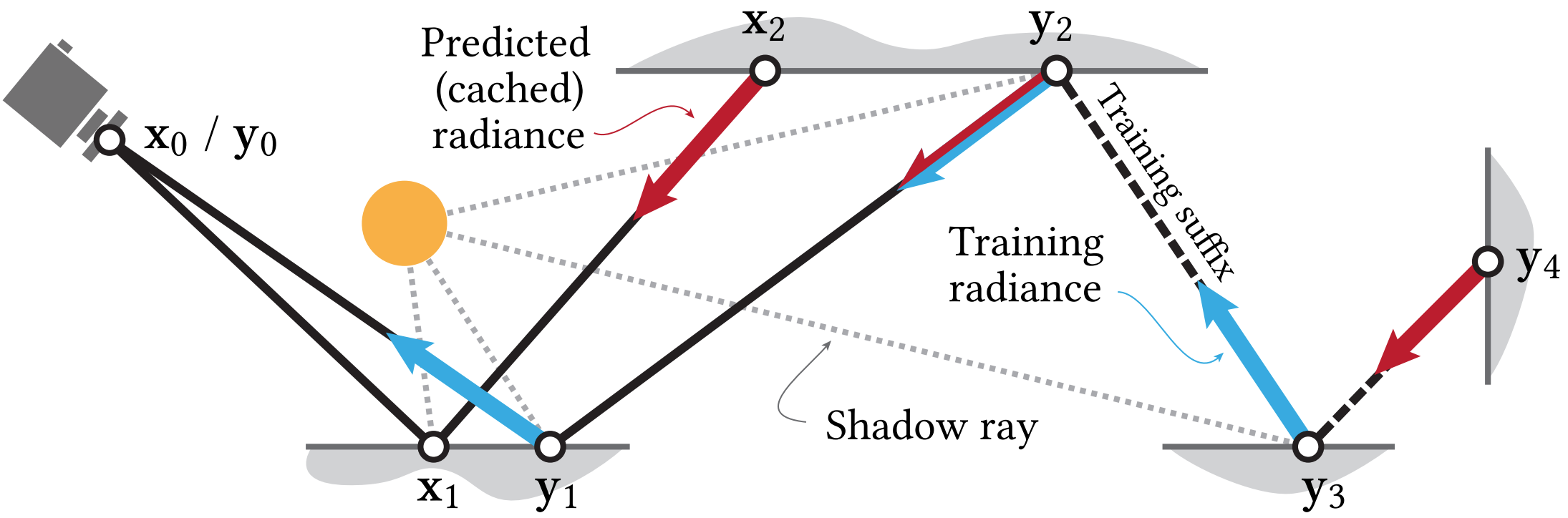
Self-Training Strategy
Instead of using noisy Monte Carlo path-traced estimates as training targets, NRC employs self-training by evaluating the neural cache itself at terminal vertices of training paths . This approach trades variance for potential bias and enables progressive simulation of multi-bounce illumination through iteration .
Each training iteration increases the number of simulated light bounces by transporting radiance learned from previous iterations . To mitigate bias, a small fraction $u = 1/16$ of training paths are made truly unbiased by terminating only via Russian roulette .
The self-training mechanism resembles Q-learning and progressive radiosity algorithms that simulate multi-bounce transport by iterating single-bounce updates .
Temporal Stabilization
To prevent temporal flickering from aggressive optimization (high learning rates and multiple gradient descent steps per frame), an exponential moving average (EMA) is applied to the network weights :
$$ \bar{W}_t := \frac{1-\alpha}{\eta_t} \cdot W_t + \alpha \cdot \eta_{t-1} \cdot \bar{W}_{t-1}, \quad \text{where } \eta_t := 1 - \alpha^t $$The parameter $\alpha = 0.99$ balances fast adaptation with temporal stability . The EMA weights $\bar{W}_t$ are used for rendering queries, while raw weights $W_t$ continue to be optimized .
Network Architecture and Input Encoding
Parameters and their encoding, amounting to $62$ dimensions: freq denotes frequency encoding [Mildenhall et al. 2020], ob denotes one-blob encoding [Müller et al. 2019], sph denotes a conversion to spherical coordinates normalized to $[0,1]^2$, and id is the identity.
| Parameter | Symbol | with Encoding |
|---|---|---|
| Position | $ \mathbf{x} \in \mathbb{R}^3 $ | $\mathrm{freq}(\mathbf{x}) \in \mathbb{R}^{3 \times 12}$ |
| Scattered dir. | $ \omega \in S^2 $ | $\mathrm{ob}(\mathrm{sph}(\omega)) \in \mathbb{R}^{2 \times 4}$ |
| Surface normal | $ \mathbf{n}(\mathbf{x}) \in S^2 $ | $\mathrm{ob}(\mathrm{sph}(\mathbf{n}(\mathbf{x}))) \in \mathbb{R}^{2 \times 4}$ |
| Surface roughness | $ r(\mathbf{x}, \omega) \in \mathbb{R} $ | $\mathrm{ob}\!\left( 1 - e^{-r(\mathbf{x},\omega)} \right) \in \mathbb{R}^{4}$ |
| Diffuse reflectance | $ \alpha(\mathbf{x}, \omega) \in \mathbb{R}^3 $ | $\mathrm{id}(\alpha(\mathbf{x},\omega)) \in \mathbb{R}^3$ |
| Specular reflectance | $ \beta(\mathbf{x}, \omega) \in \mathbb{R}^3 $ | $\mathrm{id}(\beta(\mathbf{x},\omega)) \in \mathbb{R}^3$ |
Frequency encoding ($\mathrm{freq}$) is applied to position using 12 sine functions with frequencies $2^d$, $d \in \{0, \ldots, 11\}$ . One-blob encoding ($\mathrm{ob}$) with $k=4$ evenly-spaced blobs is used for directional parameters and roughness . Diffuse and specular reflectances are passed directly ($\mathrm{id}$) .
Training Budget and Amortization
The training budget is kept stable and independent of image resolution by using a fixed number of training records per frame . Training paths are interleaved with rendering paths using a tiling mechanism: one path per tile is promoted to a training path using a random offset .
Training uses $s = 4$ batches of $l = 16384$ records each (65536 total per frame) . The tile size is dynamically adjusted to match this target budget . The training overhead is approximately 2.6ms on Full HD resolution .
Loss Function and Optimization
The network is optimized using mean squared error between predicted radiance $\tilde{L}_s(x,\omega)$ and target radiance collected from training path terminal vertices :
$$ \mathcal{L} = \frac{1}{N} \sum_{i=1}^{N} \|\tilde{L}_s(x_i, \omega_i) - L_{\text{target}}(x_i, \omega_i)\|^2 $$Four gradient descent steps are performed per frame on disjoint random subsets of training data to prevent overfitting . The high learning rate and multiple steps per frame enable rapid adaptation to dynamic scenes.
Neural Parametric Mixtures for Path Guiding
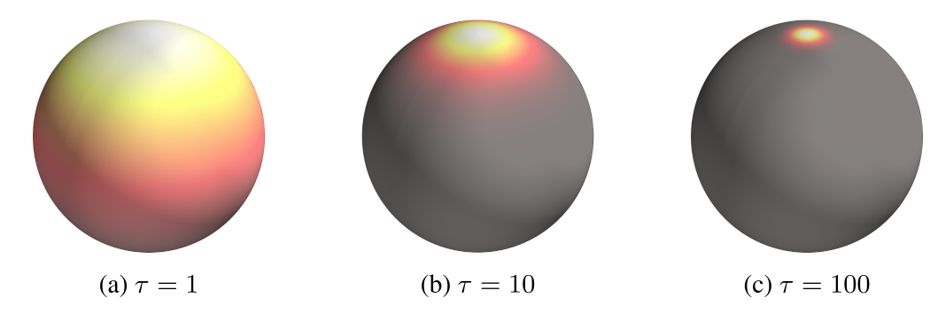
Overview
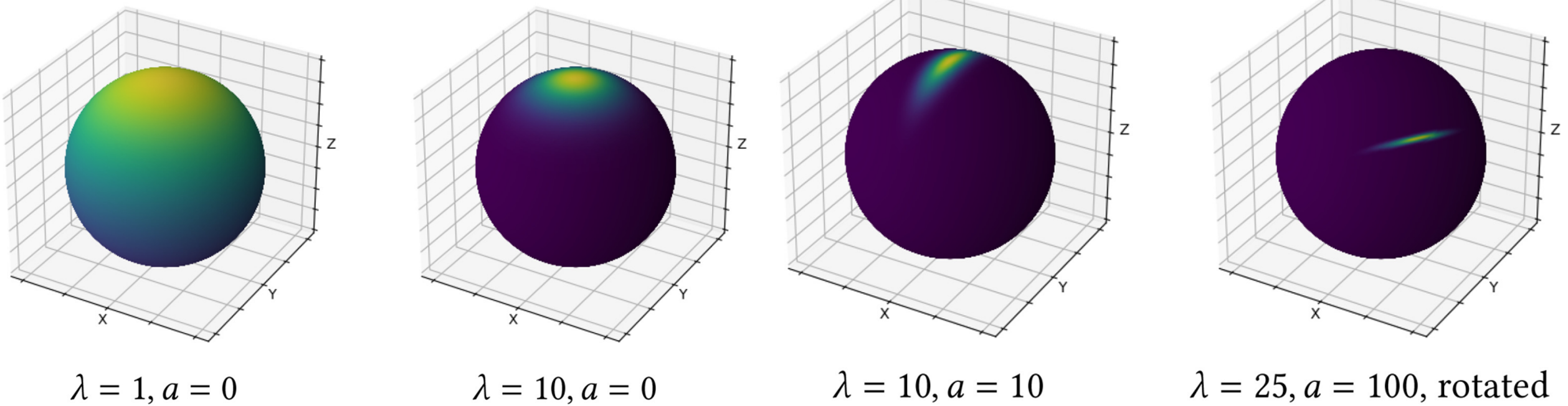
von Mises–Fisher Distribution
The vMF distribution is an isotropic probability distribution on the unit sphere $\mathbb{S}^{D-1}$, analogous to a Gaussian in $\mathbb{R}^D$.
It is parameterized by:
- Mean direction: $\mu \in \mathbb{S}^{D-1}$
- Concentration: $\kappa \in [0,\infty)$
Its PDF for direction $\omega$ is:
$$ v(\omega \mid \mu,\kappa)= C_D(\kappa)\,\exp(\kappa\,\mu^\top \omega) $$
vMF Mixture Model
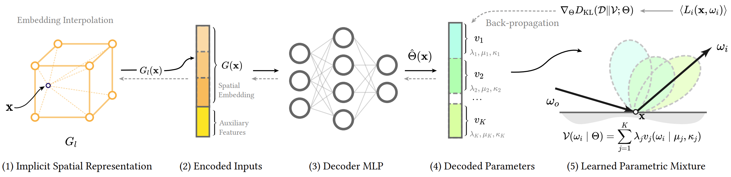
NPM predicts a mixture of $K$ vMF lobes:
$$ V(\omega \mid \Theta)= \sum_{k=1}^K \lambda_k \, v(\omega\mid\mu_k,\kappa_k). $$Mixture parameters:
- $\lambda_k \in [0,\infty)$, mixture weights
- $\sum_k \lambda_k = 1$
- $\mu_k \in \mathbb{S}^2$, mean directions
- $\kappa_k \in [0,\infty)$, concentrations
- Full parameter set:
$$ \Theta = \{ (\lambda_k,\mu_k,\kappa_k) \}_{k=1}^K $$
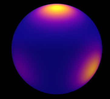
Radiance-Based NPM
Goal: make the mixture proportional to incident radiance:
$$ V(\omega_i\mid\Theta(x)) \propto L_i(x,\omega_i). $$Traditional path guiding uses kd-trees / octrees → discretization → parallax error.
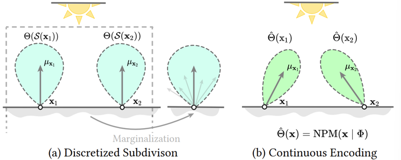
NPM instead learns a continuous implicit function:
$$ \mathrm{NPM}(x\mid\Phi)=\hat{\Theta}(x), $$where $\Phi$ are all trainable parameters (embedding + MLP).
Extended Conditioning on Outgoing Direction
For surface transport, the learned guiding distribution benefits from additionally conditioning on the outgoing direction $\omega_o$.
The extended model therefore learns
allowing the mixture parameters to adapt to view-dependent effects such as BRDF anisotropy and grazing-angle behavior.
This conditioning is implemented simply by concatenating $\omega_o$ to the MLP’s input, improving accuracy with negligible overhead.
Optimizing NPM
Raw network outputs $(\lambda'_k,\kappa'_k,\theta'_k,\phi'_k)$ are mapped into valid mixture parameters using:
| Parameter | Domain | Activation | Mapping |
|---|---|---|---|
| $\kappa_k$ | $[0,\infty)$ | Exponential | $\kappa_k=\exp(\kappa'_k)$ |
| $\lambda_k$ | $[0,\infty)$ | Softmax | $\lambda_k=\frac{\exp(\lambda'_k)}{\sum_j\exp(\lambda'_j)}$ |
| $\theta_k,\phi_k$ (spherical coords of $\mu_k$) | $[0,1]$ | Logistic | $\theta_k=\frac1{1+\exp(-\theta'_k)}$ |
Unit directions are then:
$$ \mu_k = \bigl( \sin(\pi\theta_k)\cos(2\pi\phi_k),\, \sin(\pi\theta_k)\sin(2\pi\phi_k),\, \cos(\pi\theta_k) \bigr). $$Loss: KL Divergence
Target:
$$ D(\omega)\propto L_i(x,\omega). $$KL divergence:
$$ D_{KL}(D\|V) =\int D(\omega) \log\frac{D(\omega)}{V(\omega\mid\hat{\Theta})}\,d\omega. $$Monte Carlo estimate:
$$ D_{KL}\approx \frac1N\sum_j \frac{D(\omega_j)}{p(\omega_j)} \log\frac{D(\omega_j)}{V(\omega_j)}. $$Gradient:
$$ \nabla_\Theta D_{KL}\approx -\frac1N\sum_j \frac{D(\omega_j)\,\nabla_\Theta V(\omega_j)}{p(\omega_j)V(\omega_j)}. $$Training objective:
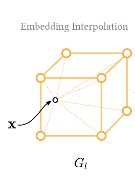
$$ \Phi^*=\arg\min_\Phi \mathbb{E}_x[D_{KL}(D(x)\|V;\Theta(x))]. $$Multi-resolution Spatial Embedding
NPM uses a learnable multi-resolution grid to encode spatial variation:
$$ \mathrm{NPM}_\Phi:x\mapsto\hat{\Theta}(x). $$A single MLP cannot represent high-frequency variation; therefore NPM uses L grids with exponentially increasing resolution.
Each grid vertex stores a trainable feature vector $\mathbf{v}\in\mathbb{R}^F$.
Querying the Embedding
For query position $x$:
- Gather the 8 neighboring grid features $V_\ell[x]$.
- Apply trilinear interpolation.
- Concatenate multi-resolution features:
Decoding Mixture Parameters
We combine the spatial embedding with auxiliary inputs (normal, roughness, $\omega_o$):
$$ \hat{\Theta}(x)= \mathrm{MLP}(G(x\mid\Phi_E)\mid\Phi_M). $$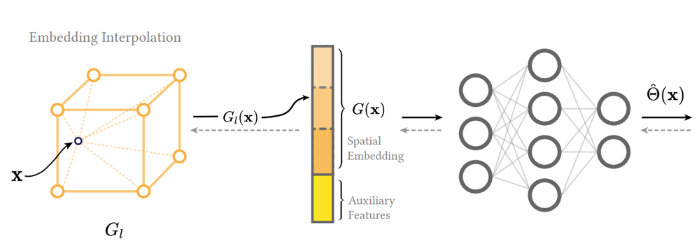
Product Distribution for Importance Sampling
During full integrand training and rendering, we sample from the product of the scattering model and the learned distribution:
$$ \boxed{ \mathcal{V}(\omega_i \mid \hat{\Theta}(x,\omega_o)) \;\propto\; f_s(x,\omega_o,\omega_i)\, L_i(x,\omega_i)\, |\cos\theta_i| } $$Equivalently, using the vMF mixture:
$$ q(\omega\mid x)\propto f_s(\omega\mid x)\,V(\omega\mid\Theta(x)). $$This aligns sampling with both the scattering function and the learned radiance.
Limitations
- vMF is isotropic; complex lobes may require many mixture components
- The number of vMF components $K$ is fixed
Online Neural Path Guiding with Normalized Anisotropic Spherical Gaussians
Overview
Fixes the limitation of vMF Mixture bwing isotropic by using Spherical Gaussians.
Limitation
- Degenerated Distributions in Certain Cases.
- Fixed components (but more expressive than vMF mixture)
Neural Product Importance Sampling via Warp Composition
Overview
Many rendering integrands take the form of a product of two functions:
$$ p^*(\omega) \propto L(\omega)\, f_r(\omega_o,\omega)\,\cos\theta , $$where
- $L(\omega)$ is the incident radiance (e.g., environment map),
- $f_r(\omega_o,\omega)$ is the BRDF,
- $\cos\theta = n \cdot \omega$ is the geometric term.
Such products are often highly multi-modal, HDR, and material dependent, making standard MIS mixtures ineffective.
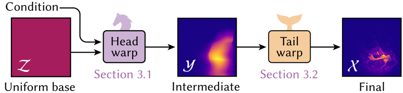
This method learns a sampler for the product distribution via a neural warp composition:
- Head warp - a conditional neural spline flow that models BRDF and cosine effects.
- Tail warp - an unconditional neural flow representing the environment map.
The decomposition reduces complexity: the tail warp embeds all lighting structure once, and the head warp learns only how the material reshapes that distribution.
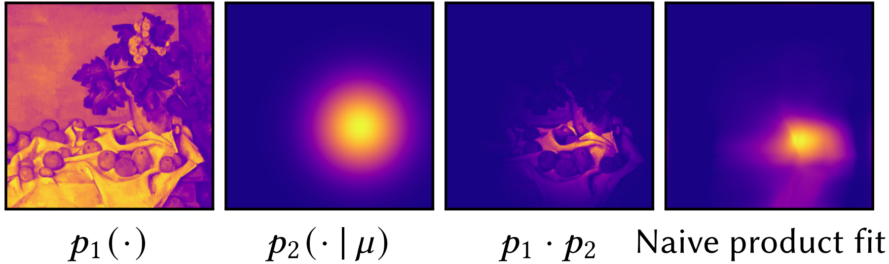
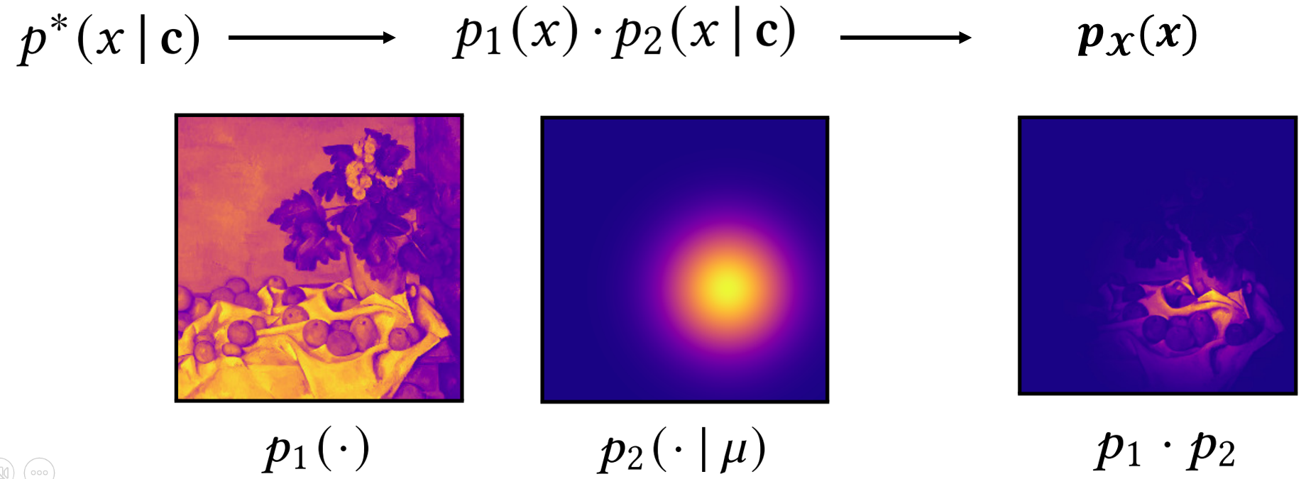
Decomposing the Product: $p_1$ and $p_2$
The product distribution is separated into two physically meaningful factors:
Emitter-driven factor
$$ p_1(\omega) \propto L(\omega), $$depending only on the environment map.
Material-driven factor
$$ p_2(\omega \mid c) \propto f_r(\omega_o,\omega)\,\cos\theta, $$where
$c = (\omega_o, n, \text{material parameters})$
is the shading condition.
The target distribution is their normalized product:
$$ p^*(\omega \mid c) \propto p_1(\omega)\, p_2(\omega \mid c). $$Intuition
- $p_1$ contains all high-frequency lighting detail (sun, HDR spots, indoor lights).
- $p_2$ contains smooth BRDF shaping (roughness, anisotropy, grazing angles).
A normalizing flow struggles to learn both simultaneously, hence the separation.
Target Distribution and Sampler
The goal is to learn a sampler
$$ \omega = T_\Phi(u, c), \qquad u \sim \text{Uniform}[0,1]^2, $$such that the induced density $p_\Phi(\omega \mid c)$ matches $p^*(\omega \mid c)$.
Neural Warp Composition
The sampler is the composition:
$$ T_\Phi = T_{\text{tail}} \circ T_{\text{head}}, $$where
- $T_{\text{head}} = h_\theta$ is the conditional head warp,
- $T_{\text{tail}} = C$ is the unconditional tail warp.
Sampling Procedure
- Sample $u \sim \text{Uniform}[0,1]^2$
- Compute $y = h_\theta(u \mid c)$
- Compute $x = C(y)$
- Map $x \in [0,1]^2$ to $\omega \in \mathbb{S}^2$ (lat-long)
The two warps handle different parts of the product.
Head Warp - Conditional Neural Spline Flow
The head warp models the BRDF × cosine factor $p_2(\omega\mid c)$.
Inputs and Conditioning
The head warp conditions on
which the encoder converts into a latent vector $\ell$.
Architecture
- Two coupling layers
- Each uses circular rational-quadratic splines (RQS)
- Spline parameters predicted from $\ell$
- Transformation: $ y = h_\theta(u \mid c), \qquad u \in [0,1]^2. $
The head warp is intentionally compact because $p_2$ is low-frequency and smooth.
Tail Warp - Environment Map Flow
The tail warp learns the mapping $x = C(y),$ such that $x$ follows the emitter distribution $p_1(\omega)$.
Training
- Trained once per environment map
- Large normalizing flow
- Encodes HDR lighting detail (spikes, sharp regions, multiple lobes)
Runtime
The tail warp is precomputed into a high-resolution lookup:
- Constant-time forward evaluation
- Stable Jacobian computation
- No conditioning
This allows head–tail composition to cleanly model the product.
Final Product Sampler
Given
the induced PDF is:
$$ p_\Phi(x \mid c)= \left| \det J_{h_\theta}(u \mid c) \right|^{-1} \left| \det J_C(y) \right|^{-1}, \qquad y = h_\theta(u \mid c). $$- $J_{h_\theta}$ and $J_C$ are the Jacobians of the head and tail flows.
- Together they approximate the ideal product
$$p^*(\omega \mid c) \propto p_1(\omega) p_2(\omega\mid c).$$
Training Objective - Forward KL
The head warp is trained (with the tail warp fixed) via forward KL divergence:
$$ \mathcal{L}_{\mathrm{KL}}(\theta)= D_{\mathrm{KL}}\!\left(p^* \,\|\, p_\Phi\right)= -\mathbb{E}_{x\sim p^*} \Big[ \log p_\Phi(x \mid c) \Big]+ \text{const}. $$Using change-of-variables:
$$ \log p_\Phi(x \mid c)=-\log \left| \det J_{h_\theta} \right|-\log \left| \det J_C \right|. $$Stabilization
An entropy regularizer encourages diverse samples and prevents mode collapse in the conditional head warp.
Limitations
- Tail warp requires training per material model for new environment map, with duration depending on conditioning dimension and target-distribution complexity
- Extremely glossy BRDFs reduce the advantage of composition
- Single-pixel sun emitters can harm tail warp smoothness
- Sometimes performs poorly when product distribution is strongly dominated by BRDF and requires MIS fallback in pathological lighting conditions
Neural Path Guiding with Distribution Factorization
Overview
The goal of path guiding is to learn a sampling distribution that approximates the target distribution:
$$ p^*(\boldsymbol{\omega} \mid \mathbf{x}) \propto f_s(\mathbf{x}, \boldsymbol{\omega}_o, \boldsymbol{\omega}) \, L_i(\mathbf{x}, \boldsymbol{\omega}) \, \cos\theta, $$where $\boldsymbol{\omega}$ is the incoming direction, $\boldsymbol{\omega}_o$ is the outgoing direction, $f_s$ is the BSDF, and $\theta$ is the angle between $\boldsymbol{\omega}$ and the shading normal.
Learning this distribution directly on the sphere is difficult because:
- The distribution varies spatially across the scene
- The distribution may be multi-modal and high-frequency
- Storage of full 2D per-voxel directional PDFs is expensive
- Interpolation of spherical PDFs is unstable
Distribution Factorization solves these issues by factorizing the directional PDF into a marginal and a conditional distribution defined on a square domain.
Hemisphere-to-Square Mapping
We map the incoming direction $\boldsymbol{\omega}$ into uniform square coordinates $(\epsilon_1, \epsilon_2) \in [0,1]^2$:
Polar coordinate:
$$ \epsilon_1 = \cos\theta \in [0,1] $$Normalized azimuth coordinate:
$$ \epsilon_2 = \frac{\phi}{2\pi} \in [0,1] $$
These coordinates can be converted to spherical domain through $\phi = 2\pi\epsilon_2$ and $\theta = \cos^{-1}(\epsilon_1)$.
Jacobian of the Mapping
The PDF defined over the uniform square space $p(\epsilon_1, \epsilon_2 \mid \mathbf{x}, \boldsymbol{\omega}_o)$ can be converted to distribution over $\boldsymbol{\omega}$, $p_\Omega(\boldsymbol{\omega} \mid \mathbf{x}, \boldsymbol{\omega}_o)$, by taking the Jacobian of the transformation into account.
Factorized Distribution Representation
We use the product rule to represent the joint PDF over the uniform square domain as:
$$ p(\epsilon_1, \epsilon_2 \mid \mathbf{x}, \boldsymbol{\omega}_o) = p_{\boldsymbol{\omega}_1}(\epsilon_1 \mid \mathbf{x}, \boldsymbol{\omega}_o) \cdot p_{\boldsymbol{\omega}_2}(\epsilon_2 \mid \epsilon_1, \mathbf{x}, \boldsymbol{\omega}_o) $$Through this representation, estimating the joint PDF boils down to predicting two 1D distributions.
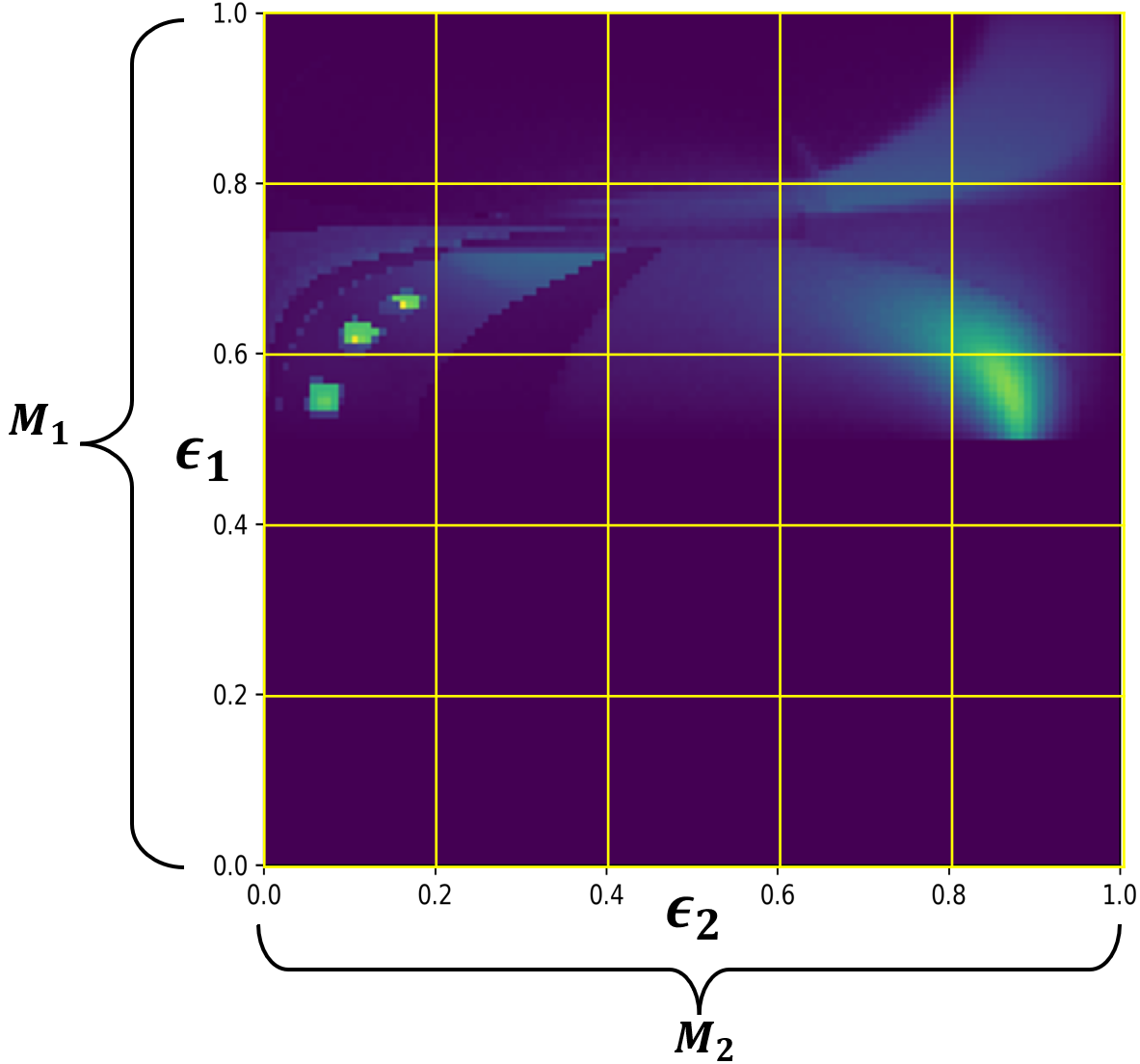
Neural Network Architecture and Discretization
We discretize the two domains $\epsilon_1$ and $\epsilon_2$ into $M_1$ and $M_2$ discrete locations, respectively, and use two independent networks to estimate the PDF at those locations.
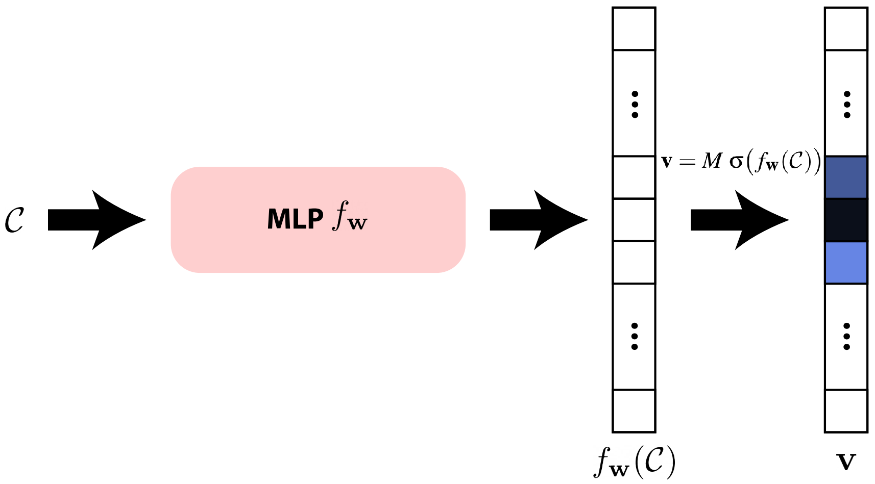
Network Structure
Marginal Network $f_{\boldsymbol{\omega}_1}$:
- Input: $\mathbf{x}$ and $\boldsymbol{\omega}_o$
- Output: An $M_1$-dimensional vector $\mathbf{v}_1$
- Function: Models $p_{\boldsymbol{\omega}_1}(\epsilon_1 \mid \mathbf{x}, \boldsymbol{\omega}_o)$
Conditional Network $f_{\boldsymbol{\omega}_2}$:
- Input: $\epsilon_1$, in addition to $\mathbf{x}$ and $\boldsymbol{\omega}_o$
- Output: An $M_2$-dimensional vector $\mathbf{v}_2$
- Function: Models $p_{\boldsymbol{\omega}_2}(\epsilon_2 \mid \epsilon_1, \mathbf{x}, \boldsymbol{\omega}_o)$
The PDF at an arbitrary location can then be obtained by interpolating the estimated PDFs at discrete locations.
Discretization Resolution
The paper sets $M_1 = 32$ and $M_2 = 16$. The reduction in resolution in the second dimension is due to the smaller angular range of $\epsilon_2$ corresponding to $\phi$ which is between 0 and $\pi$.
Network Implementation Details
The networks share the same architecture:
- Hidden layers: 3 layers with 64 neurons each
- Activation function: ReLU
To ensure valid PDFs that integrate to one, for nearest neighbor interpolation:
$$ \mathbf{v} = M \cdot \text{softmax}(f_{\boldsymbol{\omega}}(\mathbf{C})) $$where $\mathbf{C}$ is the condition (different for marginal and conditional) and $M$ is the number of bins.
Input Encoding
- Position $\mathbf{x}$: Learnable dense grid encoding
- Direction $\boldsymbol{\omega}_o$: Spherical harmonics with degree 4
- Normal and roughness: One-blob encoding using 4 bins
- Conditional input $\epsilon_1$: Triangle wave encoding with 12 frequencies for $f_{\boldsymbol{\omega}_2}$
The networks are implemented in tiny-cuda-nn.
Interpolation Strategies
The paper explores two interpolation strategies:
Nearest Neighbor
The domain is divided into $M$ bins and the PDF inside each bin is obtained from the corresponding element of the estimated vector $\mathbf{v}$:
$$ p_{\boldsymbol{\omega}}(\epsilon \mid \mathbf{C}) = \mathbf{v}[\lfloor\epsilon M\rfloor] $$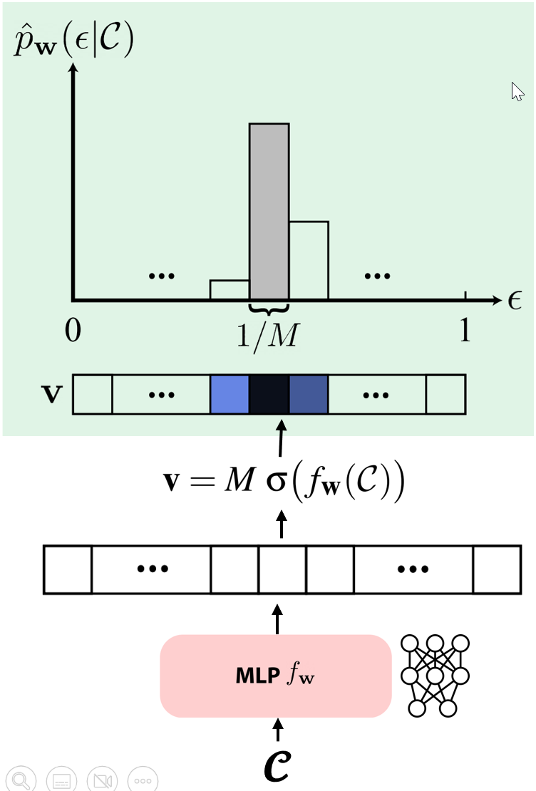
Linear Interpolation
The PDF at an arbitrary location is obtained by linearly interpolating the estimated PDF at the two nearest discrete coordinates:
$$ p_{\boldsymbol{\omega}}(\epsilon \mid \mathbf{C}) = (1-\alpha)\mathbf{v}[m] + \alpha\mathbf{v}[m+1] $$where $m = \lfloor \epsilon M - 0.5 \rfloor$ and $\alpha = \epsilon M - m - 0.5$.
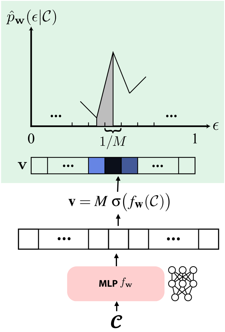
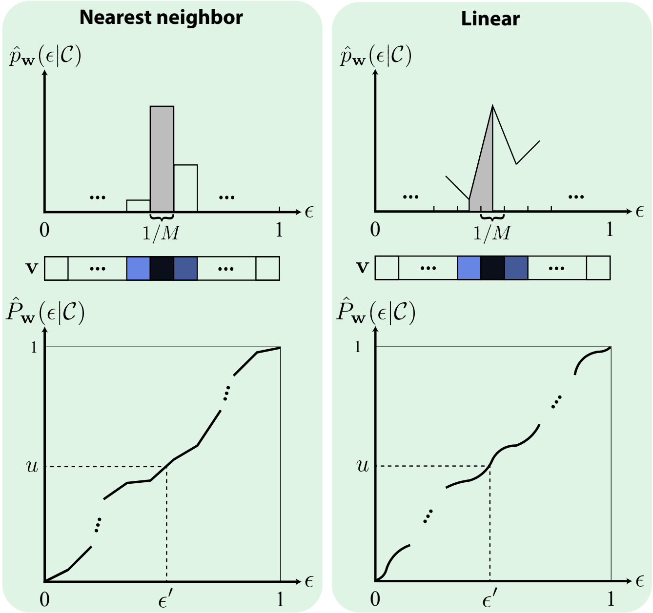
Sampling
Sampling is performed using inverse transform sampling. The inverse CDF is evaluated at a randomly generated number with uniform distribution $u \sim \mathcal{U}[0,1]$, i.e., $\epsilon = P_{\boldsymbol{\omega}}^{-1}(u \mid \mathbf{C})$.
The sampling process:
- Sample from the marginal: $\epsilon_1 = P_{\boldsymbol{\omega}_1}^{-1}(u_1 \mid \mathbf{x}, \boldsymbol{\omega}_o)$
- Sample from the conditional: $\epsilon_2 = P_{\boldsymbol{\omega}_2}^{-1}(u_2 \mid \epsilon_1, \mathbf{x}, \boldsymbol{\omega}_o)$
- Convert to spherical: $\theta = \cos^{-1}(\epsilon_1)$, $\phi = 2\pi\epsilon_2$
Optimization with Radiance Caching
The goal is to approximate the target distribution using the learned PDF by minimizing the KL divergence:
$$ D_{\text{KL}}(p^* \,\|\, p_{\boldsymbol{\Theta}}) = \int_{\Omega} p^*(\boldsymbol{\omega}) \log\frac{p^*(\boldsymbol{\omega})}{p_{\boldsymbol{\Theta}}(\boldsymbol{\omega})} \, d\boldsymbol{\omega} $$The gradient with respect to network parameters $\boldsymbol{\Theta}$ is:
$$ \nabla_{\boldsymbol{\Theta}} D_{\text{KL}}(p^* \,\|\, p_{\boldsymbol{\Theta}}) = \int_{\Omega} p^*(\boldsymbol{\omega}) \nabla_{\boldsymbol{\Theta}} \log p_{\boldsymbol{\Theta}}(\boldsymbol{\omega}) \, d\boldsymbol{\omega} $$This is approximated through MC integration:
$$ \nabla_{\boldsymbol{\Theta}} D_{\text{KL}}(p^* \,\|\, p_{\boldsymbol{\Theta}}) \approx \frac{1}{N} \sum_{i=1}^N \frac{\hat{p}^*(\boldsymbol{\omega}_i)}{q(\boldsymbol{\omega}_i)} \nabla_{\boldsymbol{\Theta}} \log p_{\boldsymbol{\Theta}}(\boldsymbol{\omega}_i) $$where samples $\boldsymbol{\omega}_i$ are drawn from $q$.
Target Distribution
The ideal target distribution is:
$$ p^*(\boldsymbol{\omega}_i \mid \mathbf{x}, \boldsymbol{\omega}_o) = \frac{f_s(\mathbf{x}, \boldsymbol{\omega}_o, \boldsymbol{\omega}_i) \, L_i(\mathbf{x}, \boldsymbol{\omega}_i) \, \cos\theta_i}{L_r(\mathbf{x}, \boldsymbol{\omega}_o)} $$where the numerator is the integrand and the denominator is the reflected radiance serving as the normalization factor.
Radiance Caching Network
To reduce the variance of gradients and estimate the normalization factor, a neural network $f_{\boldsymbol{\Phi}}$ caches the reflected radiance $L_r(\mathbf{x}', \boldsymbol{\omega}_o')$ at the next intersection point. Since $L_i(\mathbf{x}, \boldsymbol{\omega}_i) = L_r(\mathbf{x}', \boldsymbol{\omega}_o')$, this network can estimate both the incoming radiance and the normalization factor.
The estimated target distribution becomes:
$$ \hat{p}^*(\boldsymbol{\omega}_i \mid \mathbf{x}, \boldsymbol{\omega}_o) = \frac{f_s(\mathbf{x}, \boldsymbol{\omega}_o, \boldsymbol{\omega}_i) \cdot f_{\boldsymbol{\Phi}}(\mathbf{x}', \boldsymbol{\omega}_o') \cdot \cos\theta_i}{f_{\boldsymbol{\Phi}}(\mathbf{x}, \boldsymbol{\omega}_o)} $$The radiance caching approach follows Neural Radiance Caching (NRC) and uses a small MLP network that takes surface location and ray direction as input and estimates the corresponding radiance.
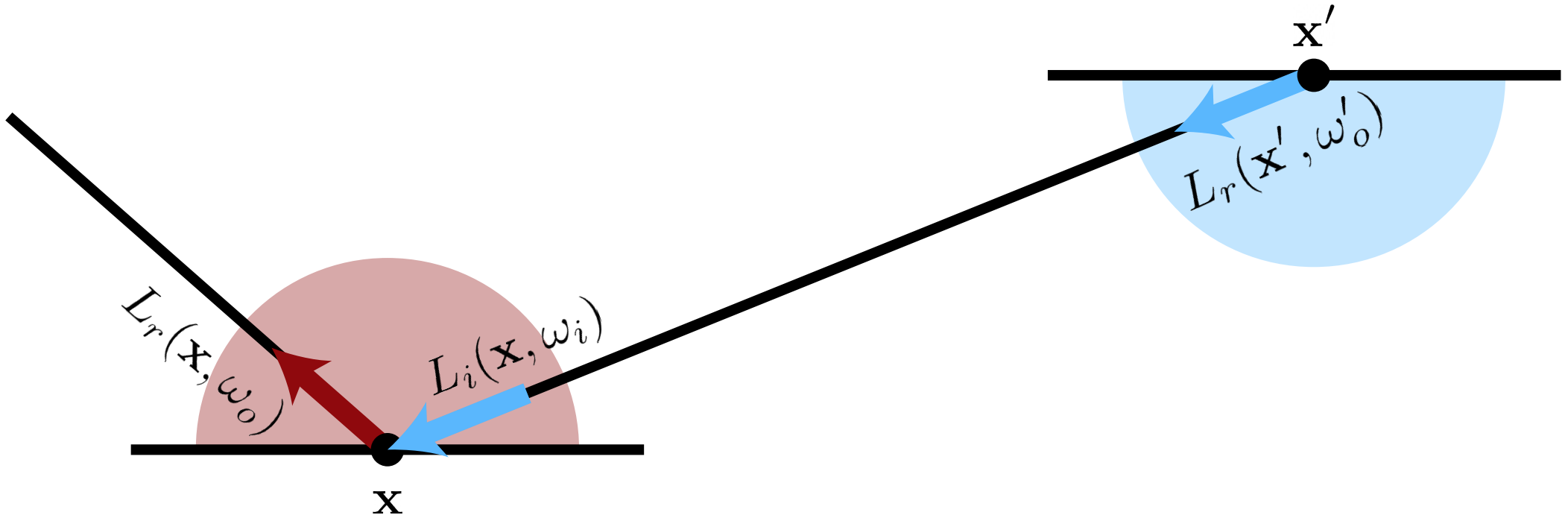
Training Details
- Training is performed in an online fashion for the first 30% of the allocated budget
- Adam optimizer with learning rate of $10^{-2}$ for $f_{\boldsymbol{\Phi}}$ and $3 \times 10^{-2}$ for $f_{\boldsymbol{\omega}_1}$ and $f_{\boldsymbol{\omega}_2}$
- 70% of paths are guided using the learned method, 30% use BSDF sampling for exploration
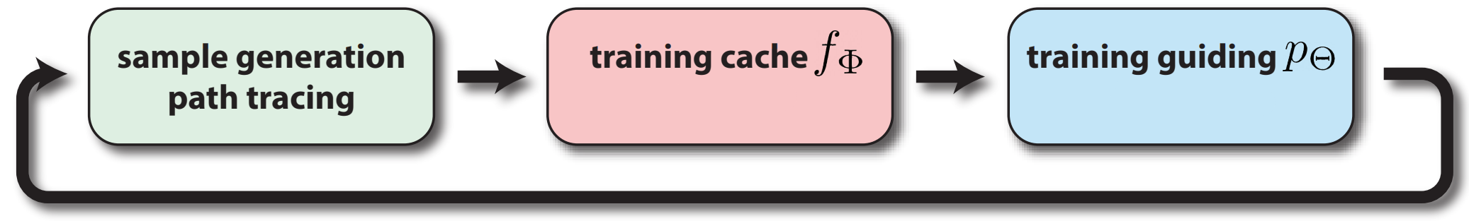
Limitations
- Uses a fixed resolution, struggling with features significantly smaller than each bin
- High-frequency distributions may require many bins
- On simple scenes with easy-to-model light transport, the advantage is not significant
References
Kajiya, James T. “The Rendering Equation.” SIGGRAPH ‘86: Proceedings of the 13th Annual Conference on Computer Graphics and Interactive Techniques, 1986.
Pharr, Matt, Wenzel Jakob, and Greg Humphreys. Physically Based Rendering: From Theory to Implementation. 3rd ed., Morgan Kaufmann, 2016. http://www.pbr-book.org.
Vorba, Jiří, Ondřej Karlík, Martin Šik, Tobias Ritschel, and Jaroslav Křivánek. “Path Guiding Using Spatio-Directional Mixture Models.” Computer Graphics Forum, vol. 33, no. 4, pp. 141-150, 2014. Presented at EGSR 2014.
Müller, Thomas, Markus Gross, and Jan Novák. “Practical Path Guiding for Efficient Light-Transport Simulation.” Computer Graphics Forum, vol. 36, no. 4, pp. 91-100, 2017. Presented at EGSR 2017.
Li, Tzu-Mao, Yu-Ting Wu, and Yung-Yu Chuang. “Offline Deep Importance Sampling for Monte Carlo Path Tracing.” Pacific Graphics, 2018.
Müller, Thomas, Markus Gross, and Jan Novák. “Neural Importance Sampling.” ACM Transactions on Graphics (TOG), vol. 38, no. 6, p. 145, 2019. Presented at SIGGRAPH 2019.
Bako, Steve, Samuli Laine, Tero Karras, Jaakko Lehtinen, and Pradeep Sen. “Real-Time Neural Radiance Caching for Path Tracing.” ACM Transactions on Graphics (TOG), vol. 40, no. 4, p. 36, 2021. Presented at SIGGRAPH 2021.
Zeltner, Tim, Shlomi Steinberg, and Wenzel Jakob. “Neural Parametric Mixtures for Path Guiding.” ACM Transactions on Graphics (TOG), vol. 42, no. 4, p. 195, 2023. Presented at SIGGRAPH 2023.
Xu, Kartic, Jiwoo Han, Ling-Qi Yan, and Ravi Ramamoorthi. “Neural Product Importance Sampling via Warp Composition.” ACM Transactions on Graphics (TOG), vol. 43, no. 6, 2024. Presented at SIGGRAPH Asia 2024.
Dahm, Kai, Lukas Hosek, Carsten Dachsbacher, and Nikolaus Binder. “Neural Path Guiding with Distribution Factorization.” Eurographics Symposium on Rendering (EGSR), 2025.
Probability Course. University of Massachusetts Amherst. https://www.probabilitycourse.com/.
Veach, Eric. Robust Monte Carlo Methods for Light Transport Simulation. PhD dissertation, Stanford University, 1997.
Owen, Art B. “Monte Carlo Theory, Methods and Examples.” https://artowen.su.domains/mc/.
TU Wien. “Rendering (VU).” Computer Graphics and Algorithms, Summer Semester 2020. https://www.cg.tuwien.ac.at/courses/Rendering/VU.SS2020.html.
KAIST CS580: Advanced Topics in Computer Graphics. “Neural Rendering.” Spring 2024. https://mhsung.github.io/kaist-cs580-spring-2024/.
Veach, Eric. Robust Monte Carlo Methods for Light Transport Simulation. PhD dissertation, Stanford University, December 1997. Available: https://graphics.stanford.edu/papers/veach_thesis/thesis.pdf