Work in Progress: This post is currently under active development.
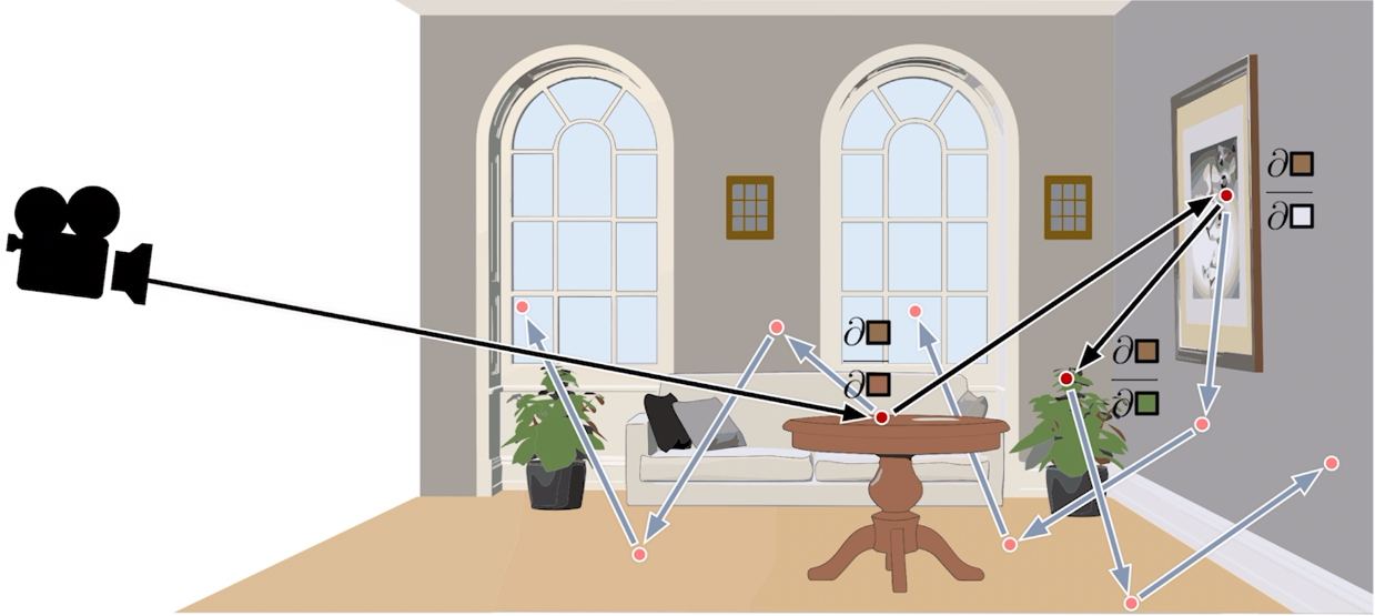
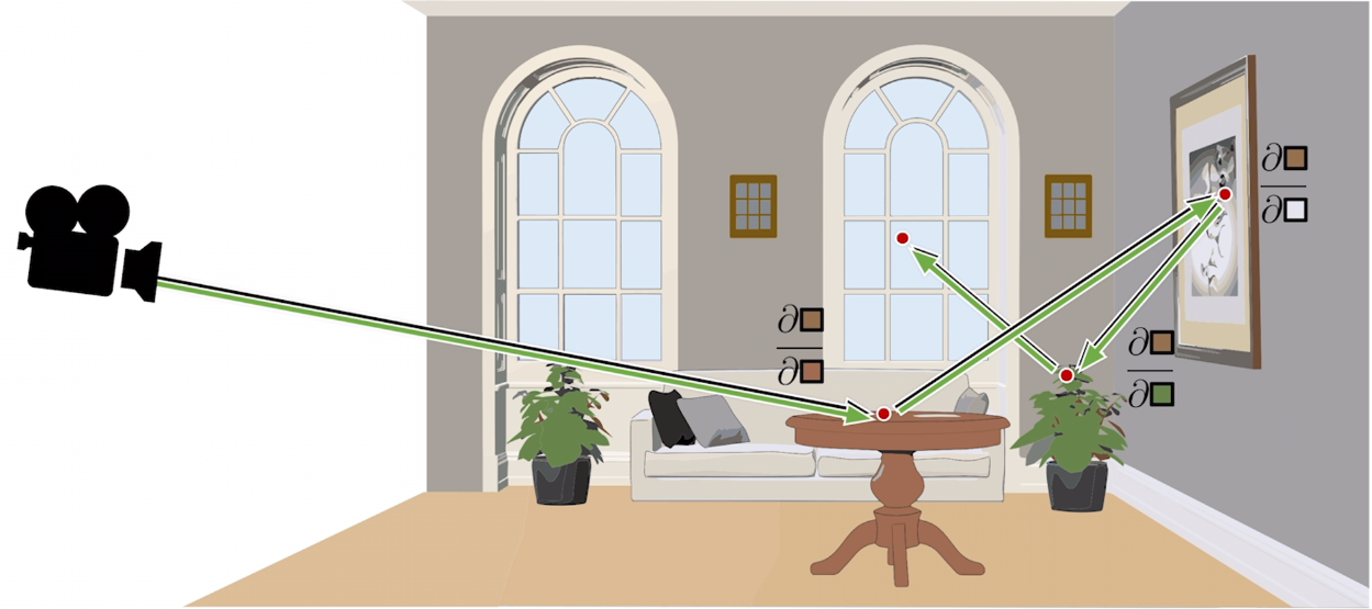
Figure 1.
High-level overview of the differentiable rendering pipeline mapping scene parameters to images and propagating loss gradients back to parameters.
Differentiable rendering asks a simple question with surprisingly sharp edges: if a renderer maps scene parameters to an image, can we differentiate that map? If yes, then geometry, materials, lights, and cameras can be optimized from image-space losses such as reconstruction error, perceptual losses, or task-specific objectives.
The difficulty is that rendering is not just a smooth program. It is an integral over paths, visibility changes discontinuously, and Monte Carlo estimators have sampling choices that may themselves depend on the parameters. This post builds the story in layers: first automatic differentiation, then why naive AD fails for visibility, then boundary-aware Monte Carlo estimators, and finally the physics-based formulations used in modern differentiable renderers.
I will assume basic familiarity with physically based rendering and the rendering equation. The goal here is not to rederive all of light transport, but to make the differentiable part clear enough that the papers become much easier to read. The main article focuses on surface transport; participating media and null-collision estimators are treated as a separate advanced topic.
The simplest approach to derivative estimation is the finite difference (FD) method. For a scalar function $f: \mathbb{R} \to \mathbb{R}$, the forward difference estimator approximates the derivative at $x$ using a small step size $h > 0$:
$$
f'(x) \approx \frac{f(x + h) - f(x)}{h}
$$
A commonly used variant is the central difference method, which provides a significantly better approximation with quadratic truncation error $\mathcal{O}(h^2)$ instead of linear $\mathcal{O}(h)$:
Finite differences are inherently biased because evaluating $f$ at a non-zero step $h$ returns a local spatial average of the true derivative rather than its point value at $x$:
where $K_h(u) = \frac{1}{2h}\mathbf{1}_{[-h,h]}(u)$ is a rectangular boxcar kernel of width $2h$. Thus, a finite difference returns a local average of $f'$ smoothed over $[-h, h]$.
This blurring can produce inaccurate gradients when $f$ contains high-frequency features or discontinuities. The bias vanishes as $h \to 0$, but infinitely small steps are numerically fragile: in floating-point arithmetic, catastrophic cancellation degrades precision, and in Monte Carlo rendering, small differences become overwhelmed by stochastic sampling noise.
It is straightforward to apply finite differences to a renderer by generating the image once with the original parameter and once with the perturbed parameter. With a Monte Carlo renderer, though, the evaluation of $f$ is noisy, and if $f(x + h)$ and $f(x)$ are evaluated independently, the FD estimator needs an enormous number of samples to converge. Using Common Random Numbers (CRN)—seeding both evaluations with identical random number generator streams—resolves this: because the Monte Carlo noise in $f(x+h)$ and $f(x)$ becomes strongly correlated, a significant portion of the variance cancels out.
Fundamentally, finite differences do not scale to functions with many input parameters due to the curse of dimensionality. For inverse rendering with a scene parameter vector $\mathbf{x} = (x_1, \dots, x_n)^T \in \mathbb{R}^n$ (such as meshes, textures, and volumes with millions of degrees of freedom), central differences would require rendering the image $2n$ times per gradient step ($f(x_1, \dots, x_i \pm h, \dots, x_n)$ for every parameter $i$). This is computationally impractical. An alternative is Simultaneous Perturbation Stochastic Approximation (SPSA), which estimates high-dimensional gradients by randomly offsetting all parameters at once.
For $f: \mathbb{R}^n \to \mathbb{R}$, SPSA estimates the gradient vector using only two function evaluations, regardless of the dimension $n$:
$$
\hat{\mathbf{g}}(\mathbf{x}) \approx \frac{f(\mathbf{x} + h \cdot \boldsymbol{\Delta}) - f(\mathbf{x} - h \cdot \boldsymbol{\Delta})}{2h} \cdot \boldsymbol{\Delta}^{-1}
$$
where $\boldsymbol{\Delta}^{-1} = (\Delta_1^{-1}, \dots, \Delta_n^{-1})^T$ denotes component-wise inversion, so each gradient component is estimated as:
$$
\hat{g}_i(\mathbf{x}) = \frac{f(\mathbf{x} + h \cdot \boldsymbol{\Delta}) - f(\mathbf{x} - h \cdot \boldsymbol{\Delta})}{2h \, \Delta_i}
$$
The random perturbation vector $\boldsymbol{\Delta}$ has entries drawn independently from a mean-zero, symmetric distribution with bounded inverse moments—in practice, almost always a Rademacher distribution (each entry $\Delta_i = \pm 1$ with equal probability). A Gaussian $\boldsymbol{\Delta}$ cannot be used here: its probability density is non-zero at $0$, so $\Delta_i^{-1}$ has infinite variance and the estimator blows up.
While SPSA requires only two function evaluations per step regardless of input dimensionality, it introduces additional stochastic direction variance into the gradient estimates. This requires careful tuning of the step size $h$ to achieve good convergence. Consequently, derivative-free methods cannot compete with gradient descent using true infinitesimal gradients computed via automatic differentiation.
Instead of approximating derivatives with finite differences or deriving a large formula by hand, we can use automatic differentiation (AD). AD runs the original computation as a sequence of simple operations and applies the chain rule to each operation. For two scalar functions, the chain rule is:
$$
\frac{d}{dx}g(f(x)) = g'(f(x))f'(x).
$$
For vector-valued functions, the same rule becomes a product of Jacobian matrices. AD evaluates the required Jacobian products without constructing the full matrices.
Figure 4.
Example computation graph corresponding to the expression $x^2 \sin(2xy)$. The edge weights are the derivative of the operation applied to the input node.
This evaluates the chain rule without finite-difference truncation error, though the computation remains subject to ordinary floating-point roundoff. Automatic differentiation was introduced between the 1950s and 1970s and later became widely used for neural network training. The following overview focuses on the parts that matter for inverse rendering. A nice implementation of this concept by Andrej Karpathy can be found on YouTube here.
Computation graphs. The central idea is to view a computation as a graph of operations. The individual operations are nodes, and the derivatives of individual steps are assigned to the graph’s edges. For example, consider:
In a computer program, we could implement the evaluation of this expression as a sequence of steps:
a=2*xb=a*yc=sin(b)d=x*xe=d*c
The corresponding computation graph is shown in Fig. . Each edge stores a local derivative. For example, because $b=ay$, the edge from $a$ to $b$ has derivative $\partial b/\partial a=y$. AD combines these local derivatives to obtain the derivative of the final output. The ordinary evaluation of the function is called the primal computation, and the saved operations are often called a tape or Wengert tape.
A key choice in AD is the direction in which derivatives move through the graph. Forward mode starts at one input and carries its derivative toward the outputs. It is most efficient when there are few inputs and many outputs.
For a function $\mathbf{y}=f(\mathbf{x})$, forward mode computes a Jacobian-vector product (JVP):
Here, $\mathbf{v}$ selects the input direction. For a scalar input $x$, we write $\partial_x a := \partial a/\partial x$ for the derivative of an intermediate value $a$. To differentiate with respect to $x$, we seed $\partial_x x=1$ and $\partial_x y=0$. Every later $\partial_x v$ is computed alongside its ordinary value $v$.
The interactive simulation below first computes $\partial e/\partial x$, then repeats the sweep for $\partial e/\partial y$:
Each forward sweep gives the derivative with respect to one chosen input. It never constructs the full Jacobian $\mathbf{J}_f$, but its cost grows with the number of inputs because the graph must be traversed again for each one. Forward mode is therefore a good fit for functions with a small number of inputs and many outputs.
Forward mode can be implemented with dual numbers. A dual number $a + \epsilon b$ stores an ordinary value $a$ and its derivative $b$, with the rule $\epsilon^2 = 0$. Multiplication then gives:
$$
(a + \epsilon b)(c + \epsilon d) = ac + \epsilon (ad + bc).
$$
The first part, $ac$, is the ordinary product. The coefficient of $\epsilon$, $ad+bc$, is exactly the product rule for its derivative. More generally, $f(a+\epsilon b)=f(a)+\epsilon b f'(a)$, so evaluating a program with dual numbers computes each value and derivative together.
The main issue with forward-mode differentiation is that the entire derivative computation needs to be carried out separately for each input variable. Similar to finite differences, this does not scale to the large number of input parameters for inverse rendering.
importmathclassDual:def__init__(self,real,dual):self.real=realself.dual=dualdef__add__(self,other):# Handle addition with a normal scalar numberother_real=other.realifisinstance(other,Dual)elseotherother_dual=other.dualifisinstance(other,Dual)else0.0returnDual(self.real+other_real,self.dual+other_dual)def__mul__(self,other):# Handle multiplication with a normal scalar numberother_real=other.realifisinstance(other,Dual)elseotherother_dual=other.dualifisinstance(other,Dual)else0.0# (a + eb) * (c + ed) = (ac) + e(ad + bc)real=self.real*other_realdual=self.real*other_dual+self.dual*other_realreturnDual(real,dual)def__rmul__(self,other):# Allows us to do 2 * Dual(...)returnself.__mul__(other)def__repr__(self):returnf"Dual(val={self.real:.4f}, grad={self.dual:.4f})"# We define a custom sine function using the dual number Taylor expansion:# sin(a + eb) = sin(a) + eb * cos(a)defdual_sin(x):ifisinstance(x,Dual):returnDual(math.sin(x.real),x.dual*math.cos(x.real))returnmath.sin(x)x=Dual(2.0,dual=1.0)# Seed the derivative here!y=Dual(3.0,dual=0.0)# The forward passa=2*xb=a*yc=dual_sin(b)d=x*xe=d*cprint("Result:",e)# Output: Result: Dual(val=-2.1463, grad=18.1062)
Reverse mode traverses the graph in the opposite direction. It starts at one output and asks how sensitive that output is to every earlier value. For the scalar output $e$, define
$$
\partial v := \frac{\partial e}{\partial v}.
$$
In this reverse-mode section, the compact symbol $\partial v$ means “the derivative of the final output $e$ with respect to $v$.” For example, $\partial x=\partial e/\partial x$. Reverse mode initializes $\partial e=1$ and propagates these derivatives backward using the chain rule. In vector notation this is a vector-Jacobian product (VJP):
A single reverse traversal computes the gradients for all inputs that affect the chosen output. This is why reverse mode is effective for inverse rendering, where millions of scene parameters contribute to one scalar loss. It is also the method used by backpropagation in neural networks.
For the graph $a=2x$, $b=ay$, $c=\sin(b)$, $d=x^2$, and $e=dc$, the complete reverse pass is:
$$
\begin{aligned}
\partial e &= 1, \\
\partial d &= (\partial e)c, & \partial c &= (\partial e)d, \\
\partial b &= (\partial c)\cos(b), \\
\partial a &= (\partial b)y, \\
\partial x &= (\partial d)2x+(\partial a)2, \\
\partial y &= (\partial b)a=(\partial b)2x.
\end{aligned}
$$
The two terms in $\partial x$ are accumulated because $x$ reaches the output through both $a$ and $d$. Notice that the final line uses $\partial b$: $y$ is an input to $b=ay$, whereas $\partial a$ already includes the separate local factor $y$.
Reverse mode is more difficult to implement because the backward pass needs values from the earlier primal computation. These values and operations are stored on the tape.
A naïve implementation that doesn’t store weights would require re-running the primal computation for every node, leading to quadratic complexity. Conversely, storing the entire graph can easily exceed system memory for complex simulations. The standard remedy is checkpointing, where the program state is only stored at a sparse set of points. Derivative terms are then recomputed locally between these checkpoints during the backward traversal. As we will see, even checkpointing is often insufficient for physically-based differentiable rendering, requiring more specialized solutions.
importmathclassVar:def__init__(self,val,_children=()):self.val=valself.grad=0.0# Store the edges of the DAGself._prev=set(_children)self._backward=lambda:Nonedef__mul__(self,other):other=otherifisinstance(other,Var)elseVar(other)# Pass (self, other) as children to the new output nodeout=Var(self.val*other.val,(self,other))def_backward():self.grad+=other.val*out.gradother.grad+=self.val*out.gradout._backward=_backwardreturnoutdef__rmul__(self,other):returnself*otherdefbackward(self):# 1. Topological sort using DFStopo=[]visited=set()defbuild_topo(v):ifvnotinvisited:visited.add(v)forchildinv._prev:build_topo(child)topo.append(v)build_topo(self)# 2. Seed the output gradientself.grad=1.0# 3. Apply chain rule to the sorted graph in reversefornodeinreversed(topo):node._backward()def__repr__(self):returnf"Var(val={self.val:.4f}, grad={self.grad:.4f})"defvar_sin(x):# Pass (x,) as the childout=Var(math.sin(x.val),(x,))def_backward():x.grad+=math.cos(x.val)*out.gradout._backward=_backwardreturnoutx=Var(2.0)y=Var(3.0)# Forward pass builds the DAG automatically in the backgrounda=2*xb=a*yc=var_sin(b)d=x*xe=d*c# A single call handles the DFS and the entire backward passe.backward()print("Result e:",e)print("Grad x:",x)print("Grad y:",y)# Output:# Result e: Var(val=-2.1463, grad=1.0000)# Grad x: Var(val=2.0000, grad=18.1062)# Grad y: Var(val=3.0000, grad=13.5016)
In many cases, symbolically differentiating a Monte Carlo estimator path tracer does not always work.
As the SIGGRAPH 2020 course notes on physically based differentiable rendering put it:
“Naïve combination of integral discretization and automatic differentiation does not compute the correct derivatives that converge in the limit.”[1]
There are two distinct reasons this happens, and we will look at both in turn: the integrand can be discontinuous in the parameter we are differentiating (the classic visibility problem), or the sampling process used to evaluate the integral can itself depend on that parameter.
However, this interchange is only valid under regularity conditions that justify differentiating under the integral sign, such as a suitable integrable bound on $\partial_\pi f$. Parameter-dependent jumps violate these conditions. In rendering, this frequently happens because of visibility: when an object moves, the color changes discontinuously across a moving boundary.
When a proposal distribution depends on the differentiated parameter, there are two valid viewpoints: detach both the generated sample and its density, or differentiate both through a parameter-independent primary sample. To compare them, consider estimating the derivative of an integral over an infinite domain.
The attached case instead draws $\xi$ from a parameter-independent uniform distribution and differentiates the complete transformed weight. It estimates the same derivative but can have different variance. Bias is introduced by mixing the two viewpoints, for example by detaching $x$ while differentiating only $1/p(x,\lambda)$ and omitting the corresponding change in sampling probability.
Example 2: Discontinuities (The Visibility Problem)#
For discontinuous integrands, the fundamental challenge is that the derivative and the integral cannot simply be swapped. Standard Monte Carlo sampling “misses” the boundary contribution entirely.
What goes wrong? The function $f(x, \pi) = (x < \pi\ ?\ 1 : 0.5)$ is a step function: constant everywhere except at the single point $x = \pi$, where it jumps. Any random sample $X$ almost surely lands away from that jump, where the derivative with respect to $\pi$ is exactly zero. The gradient information lives entirely at the moving boundary $x = \pi$, which has probability zero of being hit. So our estimator confidently returns zero every single time, while the true answer is $1/2$.
This is precisely the visibility problem in rendering: when a surface edge moves, the boundary between lit and shadowed regions shifts, but standard path tracing samples almost never land exactly on an edge. The gradient signal is invisible to naive AD.
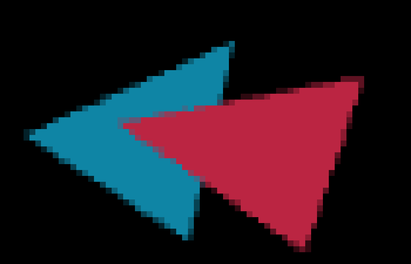
Consider a simplified rendering problem with two constant-color 2D triangles that can occlude each other. The scene parameters are the six triangle vertices ($12$ numbers) and the two RGB colors ($6$ numbers). Given these 18 values as a vector $\boldsymbol{\pi}$, with vertex parameters $\boldsymbol{\pi}_v$ and color parameters $\boldsymbol{\pi}_c$, we want to generate an image $I(\boldsymbol{\pi})$ and compute $\nabla_{\boldsymbol{\pi}} \mathcal{L}(I(\boldsymbol{\pi}))$ for an image-space loss $\mathcal{L}$.
Figure 5.
The continuous imaging function $m(x, y; \boldsymbol{\pi})$ induced by two constant-color triangles.
The triangles define an imaging function $m(x,y;\boldsymbol{\pi})$ that maps continuous image coordinates to a color according to the visible triangle. Point sampling this discontinuous function at pixel centers aliases its edges:
Figure 6.
Aliasing caused by evaluating $m(x, y; \boldsymbol{\pi})$ only at pixel centers.
Instead, each pixel $I_i$ integrates the imaging function against a reconstruction filter $k$ around its center $(x_i,y_i)$:
$$
I_i = \int \int k(x, y)m(x_i + x, y_i + y; \boldsymbol{\pi})\,dx\,dy = \int \int f(x, y; \boldsymbol{\pi})\,dx\,dy.
$$Figure 7.
Antialiasing evaluates a filtered average over each pixel support instead of one center sample.
The integral changes smoothly as a nondegenerate edge moves, even though its integrand jumps at that edge. We therefore need a differentiation rule that accounts for both changes inside the pixel support and motion of its discontinuity boundary. The next section develops exactly that rule before we return to this scene and implement its gradient.
The two failure examples and the triangle scene share one root cause: differentiating only the sampled integrand omits motion of parameter-dependent boundaries. The Leibniz rule provides the formula for differentiating an integral whose limits, as well as its integrand, depend on a parameter $\pi$.
Regularity Conditions:
One convenient set of sufficient regularity hypotheses for the Leibniz rule is the following (as detailed in standard real analysis and Delio Vicini’s PhD Thesis):
The integration limits $a(\pi)$ and $b(\pi)$ must be continuously differentiable functions of $\pi$.
The integrand $f(x, \pi)$ must be differentiable everywhere (specifically continuously differentiable, or $\mathcal{C}^1$) with respect to both $x$ and $\pi$ on the integration domain.
Under a measure-theoretic framework (using Lebesgue integration), the partial derivative $\partial f/\partial \pi$ must be Lebesgue-integrable and dominated by a Lebesgue-integrable function (enabling the use of the Lebesgue Dominated Convergence Theorem to swap differentiation and integration in the interior).
Without these hypotheses, for instance if $f$ has interior jump discontinuities that depend on $\pi$, the standard Leibniz rule cannot be applied directly.
For a 1D integral of the form $I(\pi) = \int_{a(\pi)}^{b(\pi)} f(x, \pi) dx$ satisfying these conditions, the derivative is:
$$\frac{d}{d\pi} \int_{a(\pi)}^{b(\pi)} f(x, \pi) dx = \underbrace{{\color{#00d1b2}\int_{a(\pi)}^{b(\pi)} \frac{\partial f}{\partial \pi}(x, \pi) dx}}_{\text{Interior Term}} + \underbrace{{\color{#4facfe}f(b(\pi), \pi) \frac{db}{d\pi}} - {\color{#ff6b6b}f(a(\pi), \pi) \frac{da}{d\pi}}}_{\text{Boundary Term}}$$Figure 8.
Visual decomposition of the Leibniz Integral Rule into interior and boundary components.
Proof
We can derive the general Leibniz rule in two steps: first by assuming constant boundaries, and then generalizing to variable boundaries using the multivariable chain rule.
Figure 10.
The difference in the area by evaluating $f(t+\Delta t, x) - f(t, x)$ across the integration interval with change $\Delta t$.Step 2: Cancel the original function terms
The “old” area $\int f dx$ cancels out with the negative term:
Now consider the general case where boundaries depend on time: $I(t) = \int_{a(t)}^{b(t)} f(t, x) dx$.Figure 11.
Visualization of the area under curve changed with change in the variable $\Delta t$ with limits $a(t)$ and $b(t)$
Step 1: Decompose the integration domain
We split the “new” integral $\int_{a+da}^{b+db}$ into the interior $[a,b]$ and the boundary changes:
Figure 12.
The difference in area under curve changed with change in the variable $\Delta t$ with limits $a(t)$ and $b(t)$.
Step 2: Discard higher-order terms ($O(\Delta t^2)$)
Terms like $\int \frac{\partial f}{\partial t} \Delta t dx$ in the boundary segments (which have width $\approx \Delta t$) become $\Delta t^2$ and vanish:
$$\frac{\int_a^b f dx + {\color{#00d1b2}\int_a^b \frac{\partial f}{\partial t}\Delta t dx} - {\color{#ff6b6b}\int_a^{a + a'\Delta t} f dx} + {\color{#4facfe}\int_b^{b + b'\Delta t} f dx} - \int_a^b f dx}{\Delta t}$$
Step 3: Cancel original function and evaluate boundaries
Using the Fundamental Theorem of Calculus (or Mean Value Theorem), the boundary integrals become $f(t, a) a'\Delta t$ and $f(t, b) b'\Delta t$:
$$\frac{\cancel{\int_a^b f dx} + {\color{#00d1b2}\int_a^b \frac{\partial f}{\partial t}\Delta t dx} - {\color{#ff6b6b}f(t, a)a'\Delta t} + {\color{#4facfe}f(t, b)b'\Delta t} - \cancel{\int_a^b f dx}}{\Delta t}$$
In computer graphics, we deal with 2D images and 3D scenes. The 1D Leibniz rule generalizes to higher dimensions via the Reynolds Transport Theorem (RTT).
Regularity Conditions:
As in the 1D case, a convenient sufficient set of regularity assumptions for RTT is (see Delio Vicini’s PhD Thesis [2]):
Differentiability everywhere in the subdomains: The integrand $f(\mathbf{x}, \pi)$ must be continuously differentiable ($\mathcal{C}^1$) with respect to both $\mathbf{x}$ and $\pi$ everywhere in the interior of the domains separated by the boundary/discontinuity surfaces $\Gamma(\pi)$.
Lipschitz Continuity: The boundary motion mapping (the trajectory of boundary points $\mathbf{x}(\pi)$) is Lipschitz continuous, so the boundary velocity field $\partial_\pi \mathbf{x}$ exists almost everywhere.
Lebesgue-Integrability: Both the integrand $f(\mathbf{x}, \pi)$ and the partial derivative $\partial_\pi f(\mathbf{x}, \pi)$ must be Lebesgue-integrable over the respective interior domains.
For an integral over a moving domain $X(\pi)$ satisfying these conditions:
$X(\pi)$ is the integration domain, which moves as $\pi$ changes.
$\Gamma(\pi)$ is the full boundary: the union of the external boundary $\partial X(\pi)$ and
any internal surfaces where $f$ is discontinuous (e.g. silhouette edges of objects).
On an internal interface, $\mathbf{n}$ is a consistently chosen unit normal pointing from the minus side to the plus side; on the external boundary it is outward-facing.
$\partial_\pi \mathbf{x}$ is the velocity of the boundary: how fast each boundary point moves
as $\pi$ changes.
$\Delta f(\mathbf{x}, \pi) = f^-(\mathbf{x}) - f^+(\mathbf{x})$ is the jump in $f$ across
$\Gamma$, with $f^-$ on the side from which $\mathbf n$ points and $f^+$ on the side toward
which it points. On an external boundary, take the outside value $f^+$ to be zero.
Note that for points on $\Gamma$ where $f$ is actually continuous, $\Delta f = 0$ and they
contribute nothing to the boundary integral, so it is safe to include more boundary points than
strictly necessary. This matters in practice: when rendering, we do not always know in advance
which edges are true silhouettes, so we can include all triangle edges and let the $\Delta f$
term naturally zero out the non-contributing ones.
This is the key formula for differentiable rendering. It tells us that the standard interior derivative
must be supplemented with the boundary contribution. Explicit edge sampling evaluates this term
directly; reparameterization and warped-area methods convert it into an equivalent interior estimator.
Continuing Example 2, let’s see how this
resolves the failure of naïve AD. The function is:
$$
I(\pi) = \int_0^1 f(x, \pi)\, dx, \quad \text{where } f(x, \pi) = \begin{cases} 1 & \text{if } x < \pi \\ 0.5 & \text{if } x > \pi \end{cases}
$$Figure 13.
Visualization of the step function $f(x, \pi)$ with a discontinuity at $x = \pi$.
The discontinuity is at $x = \pi$, so $\Gamma = \{\pi\}$, $\langle \partial_\pi x, \mathbf{n} \rangle = 1$,
and the jump is $\Delta f = f^-(\pi) - f^+(\pi) = 1 - 0.5 = 0.5$. Applying the 1D Leibniz rule:
This matches the analytic derivative of $I(\pi) = 0.5\pi + 0.5$, confirming $\frac{dI}{d\pi} = 0.5$.
Unlike naive AD, which returns zero by only seeing the interior term, the Leibniz rule correctly
captures the contribution of the moving discontinuity by explicitly accounting for the jump
$\Delta f$ at the boundary.
We now return to the filtered triangle image introduced above. We will not discuss the choice of reconstruction filter $k$ here; the PBRT book provides a detailed treatment of reconstruction filters.
Most renderers, whether real-time, offline, physics-based, differentiable or not, need to deal with the aliasing issue. Most of them solve the antialiasing integral numerically by evaluating the imaging function at sample locations. For a unit-area pixel and uniformly distributed or suitably equidistributed samples, the approximation is:
where $(x_j, y_j)$ are sample locations within the $i$-th pixel. For a nonuniform density $p$, each summand instead carries the importance weight $f(x_j,y_j)/p(x_j,y_j)$. The naive approach of evaluating at the pixel center can also be seen as a one-point quadrature rule with $N = 1$ and $x_1 = y_1 = 0.5$.
We say a discretization is consistent if it converges to the integral, i.e., $\lim_{N\rightarrow \infty} \frac{1}{N} \sum_{j=1}^N f(x_j, y_j; \boldsymbol{\pi}) = I_i$ under the unit-area uniform-sampling convention above. The samples need not be stochastic, but a deterministic sequence must still induce the correct integration measure. If the points are sampled uniformly at random, the estimator is unbiased when $\mathbb{E}[f(x_j, y_j)] = I_i$.
Integration is not limited to antialiasing. Motion blur integrates over the time for which the shutter is open, defocus blur integrates over the lens aperture, and area-light illumination integrates over the light source. The rendering equation similarly expresses global illumination through recursive integration over light-scattering directions.
Remember that our goal is to differentiate a scalar loss $\mathcal{L}$ with respect to the scene-parameter vector $\boldsymbol{\pi}$. The chain rule gives:
Here, $\partial \mathcal{L}/\partial I_i$ measures how the loss responds to pixel $i$, while $\nabla_{\boldsymbol{\pi}} I_i$ measures how that pixel responds to every scene parameter. For a fixed target image $\hat{I}$, a pixel-wise squared loss is
We therefore need the derivative of each pixel color with respect to the scene parameters.
Figure 14.
A pixel support overlapping triangle boundaries. We want the derivative of the filtered pixel color with respect to vertex positions.
A common misconception is that a discontinuous visibility function makes the filtered pixel value non-differentiable everywhere. Recall that $I_i$ averages color over the filter support. Away from degenerate events such as topology changes or coincident edges, moving a triangle changes this average smoothly. The rendering integrand can be discontinuous even when its integral is differentiable. Rendering was not turned into an integral merely to obtain this property; image formation is already an integration problem, and rendering algorithms are numerical approximations of that integral.
How do we compute the derivatives of an integral? Recall that we wanted to compute the integral numerically (Equation $\eqref{eq:discretization}$). Unfortunately, we cannot just automatically differentiate the numerical integrator as we saw in Example 2. For vertex-position parameters and samples away from edges, naive AD returns a zero derivative almost surely.
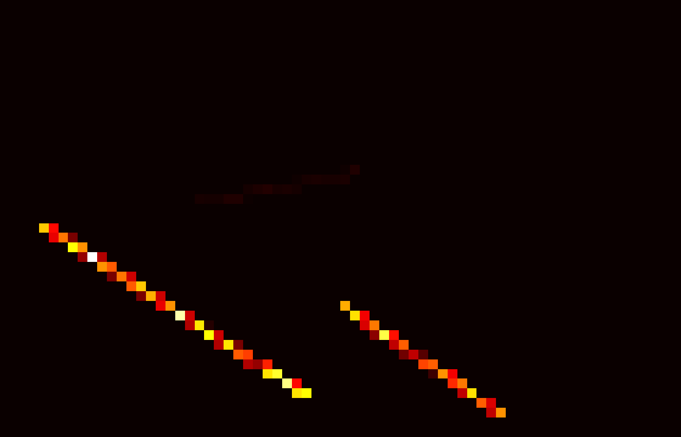
Figure 15.
Samples away from the boundary see a locally constant color, so naive AD returns zero even though the filtered pixel changes.
However, the derivative of the integral with respect to a vertex position parameter $\mathbf{\pi}_v$ is not 0.
This is the same failure mode as Example 2: the discretization and the gradient operator do not commute for discontinuous integrands, since a uniformly placed sample has zero probability of landing exactly on the moving edge where the change actually happens. The fix is also the same one, sample the boundary explicitly.
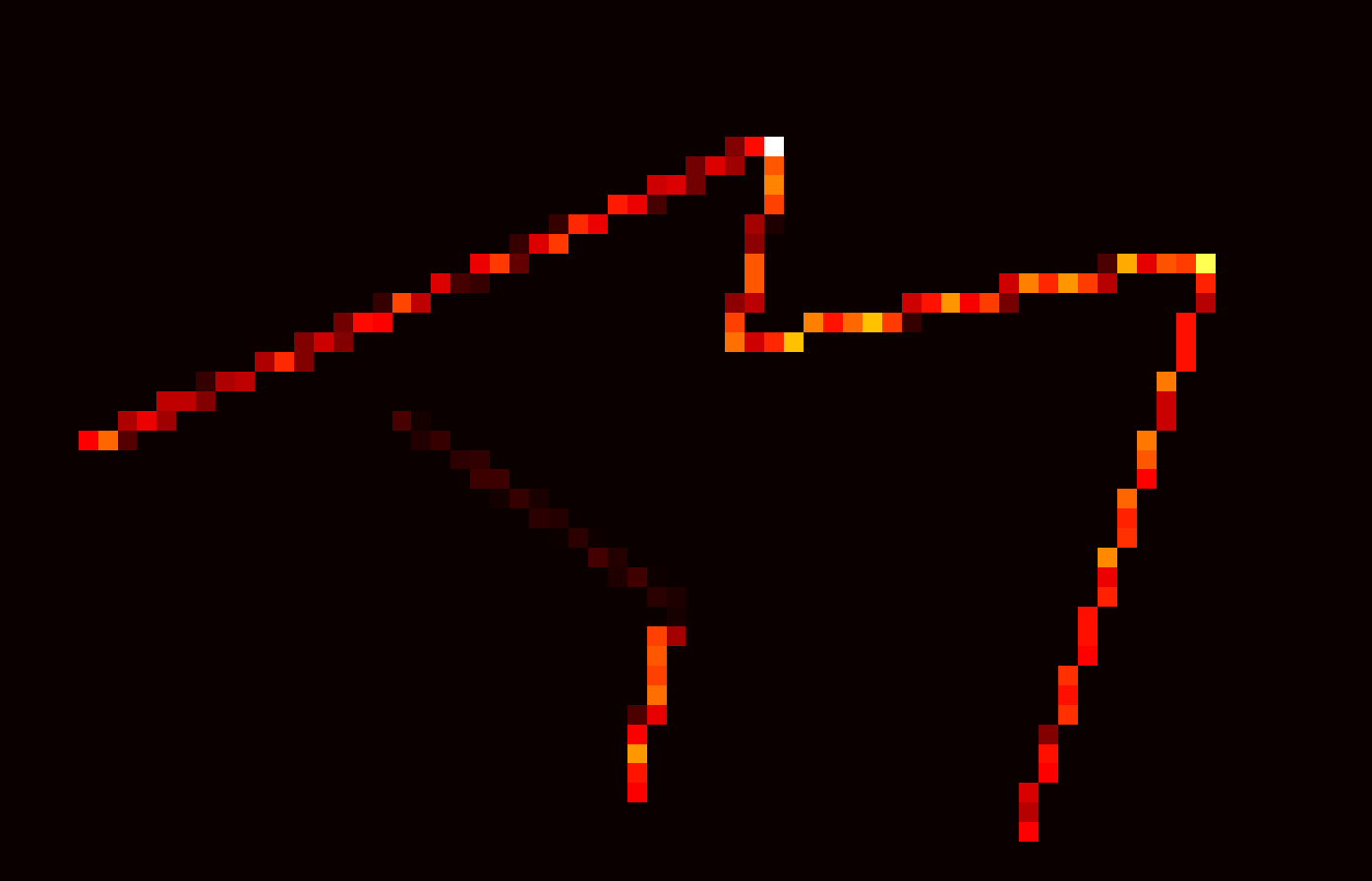
Figure 16.
Sampling the boundary captures the missing gradient contribution from moving visibility edges.
In general, we need to evaluate the Reynolds Transport Theorem (Equation $\eqref{eq:reynolds-transport-theorem}$) for this problem:
Figure 17.
The Reynolds Transport Theorem decomposed into interior and boundary derivatives.
To intuitively understand the boundary derivative, we can visualize it as calculating the volume of an infinitesimal boundary wedge created by the movement of an edge.
For every point on a silhouette edge, as the parameter $\pi$ changes, the edge sweeps out a small parallelogram. The boundary integral accumulates these infinitesimal volumes along the entire discontinuity contour.
We can decompose the integrand into three intuitive geometric components:
Height ($f_- - f_+$): The difference in pixel color (or radiance) between the two sides of the edge (e.g., transitioning from the occluded blue background to the moving red foreground).
Width ($n \cdot v$): The distance the edge moves, projected along the normal direction $n$. Movement parallel to the edge simply slides along the boundary and doesn’t change the area; only perpendicular movement contributes to the derivative!
Length ($ds$): The differential line element along the boundary contour.
which can also be approximated with Monte Carlo sampling.
Figure 18.
The Infinitesimal Boundary Volume. For each point on the boundary, we compute its 2D movement $v$ with respect to the differentiating parameter. This movement is projected onto the normal direction $n$ to yield the normal movement speed $n \cdot v$. This projection accounts for the infinitesimal width of the swept area, allowing us to properly measure the infinitesimal area changes at the boundary. Multiplying this projected width by the differential edge segment $dt$ (length) and the color jump (height) calculates the exact boundary derivative contribution.
The following code is adapted from SIGGRAPH 2020 Course.
importnumpyasnpclassTriangleMesh:def__init__(self,vertices,indices,colors):self.vertices=np.array(vertices,dtype=np.float64)# (N, 2) verticesself.indices=np.array(indices,dtype=np.int32)# (M, 3) face indicesself.colors=np.array(colors,dtype=np.float64)# (M, 3) per-face RGBdefraytrace(mesh,pos):"""
Uses the half-plane test: a point is inside a triangle if it's
on the same side of all three edges.
"""foriinrange(len(mesh.indices)):# Extract the current triangleidx=mesh.indices[i]v0,v1,v2=mesh.vertices[idx[0]],mesh.vertices[idx[1]],mesh.vertices[idx[2]]# Edge normals (2D perpendicular: normal of (dx,dy) = (-dy, dx))defnormal_2d(v):returnnp.array([-v[1],v[0]])# Get edge normals for all edges of trianglesn01=normal_2d(v1-v0)n12=normal_2d(v2-v1)n20=normal_2d(v0-v2)# Find in which side pos is for each edgeside01=np.dot(pos-v0,n01)>0side12=np.dot(pos-v1,n12)>0side20=np.dot(pos-v2,n20)>0# if it is on same side for all edges, then it is inside (since this is 2D)if(side01andside12andside20)or(notside01andnotside12andnotside20):returnmesh.colors[i],ireturnnp.array([0.0,0.0,0.0]),-1# backgrounddefrender(mesh,h,w,spp=4):"""
Forward pass: render the mesh into an image.
"""img=np.zeros((h,w,3))# setup the (H, W, 3) buffer for RGB imagesqrt_spp=int(np.sqrt(spp))# grid cells for stratified sampling# For each pixelforyinrange(h):forxinrange(w):# for each grid cellfordyinrange(sqrt_spp):fordxinrange(sqrt_spp):# Offset the position within the pixelxoff=(dx+np.random.rand())/sqrt_sppyoff=(dy+np.random.rand())/sqrt_spp# compute the color at that positionpos=np.array([x+xoff,y+yoff])color,_=raytrace(mesh,pos)img[y,x]+=color/sppreturnimgdefcompute_interior_derivatives(mesh,adjoint,spp=4):"""
Interior derivatives: ∂Loss/∂color.
Standard AD works here because color changes are continuous.
"""img_h,img_w=adjoint.shape[:2]sqrt_spp=int(np.sqrt(spp))d_colors=np.zeros_like(mesh.colors)# For each pixelforyinrange(img_h):forxinrange(img_w):# For each grid cellfordyinrange(sqrt_spp):fordxinrange(sqrt_spp):# Find the position within the cell within pixelxoff=(dx+np.random.rand())/sqrt_sppyoff=(dy+np.random.rand())/sqrt_spp# compute the gradient at that positionpos=np.array([x+xoff,y+yoff])_,hit_idx=raytrace(mesh,pos)ifhit_idx>=0:d_colors[hit_idx]+=adjoint[y,x]/sppreturnd_colorsdefcollect_edges(mesh):"""Collect unique edges."""edges=set()# Stores edges as tuples (u, v)foridxinmesh.indices:edges.add((min(idx[0],idx[1]),max(idx[0],idx[1])))edges.add((min(idx[1],idx[2]),max(idx[1],idx[2])))edges.add((min(idx[2],idx[0]),max(idx[2],idx[0])))# [(u, v) ...]returnlist(edges)defbuild_edge_sampler(mesh,edges):"""Build CDF for importance-sampling edges by length."""lengths=[]# Store the lengths of the edgesforv0_id,v1_idinedges:lengths.append(np.linalg.norm(mesh.vertices[v1_id]-mesh.vertices[v0_id]))lengths=np.array(lengths)# Use the edge lengths as weight for PDF and construct CDFpmf=lengths/lengths.sum()cdf=np.concatenate([[0],np.cumsum(pmf)])returnpmf,cdf,lengthsdefcompute_edge_derivatives(mesh,adjoint,n_edge_samples=10000):"""∂Loss/∂vertices via Reynolds Transport Theorem."""# Extract unique edges and build CDF for samplingimg_h,img_w=adjoint.shape[:2]edges=collect_edges(mesh)pmf,cdf,lengths=build_edge_sampler(mesh,edges)d_vertices=np.zeros_like(mesh.vertices)screen_dx=np.zeros((img_h,img_w,3))screen_dy=np.zeros((img_h,img_w,3))foriinrange(n_edge_samples):# 1. Pick an edge (importance sampling by length)u=np.random.rand()edge_id=np.searchsorted(cdf,u,side='right')-1edge_id=np.clip(edge_id,0,len(edges)-1)u,v=edges[edge_id]# 2. Pick a point on the edgev0=mesh.vertices[u]v1=mesh.vertices[v]t=np.random.rand()# t in [0, 1]p=v0+t*(v1-v0)xi,yi=int(p[0]),int(p[1])ifxi<0oryi<0orxi>=img_woryi>=img_h:continue# 3. Sample both sides of the edge (the "jump" / discontinuity)edge_dir=(v1-v0)/np.linalg.norm(v1-v0)n=np.array([-edge_dir[1],edge_dir[0]])# outward normaleps=1e-3color_in,_=raytrace(mesh,p-eps*n)color_out,_=raytrace(mesh,p+eps*n)# 4. Compute gradient contribution (Reynolds Transport Theorem)pdf=pmf[edge_id]/lengths[edge_id]weight=1.0/(pdf*n_edge_samples)color_diff=color_in-color_out# the jump Δfadj=np.dot(color_diff,adjoint[yi,xi])# dp/dv0 = (1-t), dp/dv1 = t (from p = v0 + t*(v1-v0))d_v0=np.array([(1-t)*n[0],(1-t)*n[1]])*adj*weightd_v1=np.array([t*n[0],t*n[1]])*adj*weightd_vertices[u]+=d_v0d_vertices[v]+=d_v1# Screen-space derivativesscreen_dx[yi,xi]+=-n[0]*color_diff*weightscreen_dy[yi,xi]+=-n[1]*color_diff*weightreturnd_vertices,screen_dx,screen_dy# 1. Scene setupc_blue=[15/255,133/255,165/255]c_red=[187/255,37/255,66/255]scale=2.0mesh=TriangleMesh(vertices=np.array([# Tri 0 (Red)[10.0,12.0],[26.0,1.0],[31.0,16.0],# Tri 1 (Blue)[2.0,11.0],[16.0,2.0],[20.0,19.0],])*scale,indices=[[0,1,2],[3,4,5]],colors=[c_red,c_blue])# Window setupW,H,spp=70,45,4np.random.seed(48)# 2. Forward Passprint("Rendering...")img=render(mesh,H,W,spp)# 3. Backward Pass (Interior: ∂I/∂color)adjoint=np.ones((H,W,3))# Uniform adjoint to pull gradientsd_colors=compute_interior_derivatives(mesh,adjoint,spp)# 4. Backward Pass (Edges: ∂I/∂vertex via boundary sampling)d_verts,screen_dx,screen_dy=compute_edge_derivatives(mesh,adjoint,n_edge_samples=W*H)print("\nVertex Gradients (d_verts):")print(np.round(d_verts,4))# Output:# Vertex Gradients (d_verts):# [[ -4.2248 2.533 ]# [ 7.4785 -18.8305]# [ 13.7454 13.4763]# [-21.0542 4.3572]# [ 0.4232 -20.9386]# [ 2.0691 19.6481]]
While explicitly finding and sampling edges works well for 2D triangles, doing this for complex 3D meshes with secondary bounces such as shadows and reflections is much harder. We now turn to estimators designed for full Monte Carlo light transport.
where $g$ is an image-based objective function. To simplify the notation, we will consider only the intensity $I$ of a single pixel $j$ and one differentiable parameter $\pi$. The derivations generalize to differentiable rendering of RGB images and multiple parameters.
As in the two-triangle example above, the outermost step is just the chain rule. What’s new this time is that $I$ itself will be estimated by noisy Monte Carlo samples rather than computed exactly, and we need to handle that carefully. Using the simplified notation, our goal is to compute the derivative $\partial_\pi g(I(\pi))$. The chain rule allows writing this term as:
where $g'$ is the derivative of the objective function. We further declutter the notation by dropping the explicit dependency of $I$ on $\boldsymbol{\pi}$ from now on. We use Monte Carlo integration to estimate $I$. If we replace $I$ with a Monte Carlo estimator $\hat{I}$ in the equation above and take the expected value we get:
Generally, this is not an unbiased estimator of the true objective gradient. One source of bias is that $g'(\hat{I})$ and $\partial_{\boldsymbol{\pi}} \hat{I}$ use the same random samples, producing the covariance term. We can remove that covariance term, provided the random streams are independent, by using a primal estimator $\hat{I}^p$ for $g'$ and a separate derivative estimator $\partial_{\boldsymbol{\pi}} \hat{I}^a$:
In practice, this means rendering two images with independent random number streams. For nonlinear $g$, a second plug-in bias can remain because $\mathbb{E}[g'(\hat I^p)]$ need not equal $g'(I)$; increasing the primal sample count reduces this bias.
The remaining challenge is to estimate $\partial_{\boldsymbol{\pi}} I$ itself. The following derivation assumes that the integrand has no $\boldsymbol{\pi}$-dependent discontinuities. Mathematically, we need to differentiate a parameter-dependent, high-dimensional integral over light paths:
Here, a path $\mathbf{x}=(\mathbf{x}_0,\ldots,\mathbf{x}_k)$ is a sequence of sensor, surface, and emitter vertices, and $\mathcal{P}$ denotes the union of these path spaces over possible lengths $k$. A renderer also makes discrete choices, including path length, light or BSDF lobe selection, and Russian roulette; we return to those choices below. The function $f$ is the parameter-dependent contribution of a path. If $f$ does not contain parameter-dependent discontinuities, we can directly estimate its derivative using Monte Carlo integration. The derivative operator can be moved into the integral:
For this estimator, we need to differentiate the evaluation of $f$. We do not have to differentiate the sampling process that produces $\mathbf{x}_i$ or the corresponding PDF $p(\mathbf{x}_i)$. We call this estimator detached since both sampling and PDF evaluation are detached from the differentiation process. This is the most commonly used estimator in differentiable rendering. Zeltner et al. (2021) [12] provide the systematic study of this attached/detached distinction that the next two subsections summarize.
If $f$ contains $\boldsymbol{\pi}$-dependent discontinuities, additional precautions are required (e.g., edge sampling or reparameterization). Similarly, if the path space $\mathcal{P}$ is parameter-dependent, we need to account for changes in its geometry or switch to a parameterization of the integration domain that is independent of $\boldsymbol{\pi}$.
While conceptually simple, the detached estimator does not handle all potential use cases. In particular, it does not support perfectly specular BSDFs. Such BSDFs are delta functions, which do not yield valid derivatives. The solution to this problem is to also differentiate the BSDF sampling process. By doing so, we switch from differentiating the integrand by itself to differentiating the ratio of integrand to PDF. This avoids having to differentiate the delta function of the specular BSDF, as it cancels out with the sampling density.
Differentiating the sampling process can be interesting beyond perfectly specular surfaces. Many of the sampling steps in a Monte Carlo renderer are highly scene-dependent. For example, the roughness parameter of a microfacet BSDF will affect the sampling of the scattered direction. This and other sampling methods usually transform a set of uniformly distributed random numbers to the desired target distribution, e.g., using inverse transform sampling. We can interpret this transformation as a reparameterization of the original integral.
Because the sampling strategy may produce different distributions depending on the parameter $\boldsymbol{\pi}$, this choice also affects the variance properties of the resulting gradient estimator.
Formally, sampling strategies can be understood as a change of variables to new coordinates $\mathbf{u} \in \mathcal{U}$ parameterizing the integration domain $\mathcal{P}$ via a mapping $\mathcal{T} : \mathcal{U} \to \mathcal{P}$, where $\mathcal{U} =[0, 1]^n$ is a unit-sized hypercube of suitable dimension. The space $\mathcal{U}$ is called the primary sample space. The mapping $\mathbf{x} = \mathcal{T}(\mathbf{u})$ is constructed from a target density $p(\mathbf{x})$ so that its Jacobian determinant satisfies $|J_\mathcal{T}(\mathbf{u})| = p(\mathbf{x})^{-1}$. The reparameterized integral then takes the form:
This formulation is called attached, since samples geometrically follow the motion of $\mathcal{T}(\mathbf{u}, \boldsymbol{\pi})$ with respect to perturbations of $\boldsymbol{\pi}$. Similar to before, we can build an estimator of the derivative by applying Monte Carlo integration:
The attached estimator is primarily useful for perfectly specular surfaces, but it can also produce lower variance than the detached version for derivatives of BSDFs with low roughness. On the other hand, the additional motion of the samples might introduce more variance in the evaluation of other terms in the integrand.
Attached sampling handles a local delta interaction when the sampled specular direction changes smoothly with the scene parameters. It does not by itself resolve discontinuous visibility through a chain of specular events or changes in caustic-path topology. Those cases require specialized path-space or manifold techniques and are outside the surface-visibility methods developed here.
Finally, the attached estimator is more difficult to use as in practice it requires handling discontinuities in the sampling function $\mathcal{T}$. Examples of such discontinuities are discrete sampling decisions such as in delta tracking or discontinuities due to sampled rays hitting different objects as $\boldsymbol{\pi}$ changes.
Question
Detached estimator
Attached estimator
What is differentiated?
The path contribution $f$
The complete sample weight $f/p$ and continuous sampling map $\mathcal{T}$
Do samples move with $\boldsymbol{\pi}$?
No
Yes, through $\mathcal{T}(\mathbf{u},\boldsymbol{\pi})$
Typical use
Smooth finite-valued BSDFs and emission
Delta BSDFs and low-roughness sampling
Main difficulty
Misses parameter-dependent boundaries
Sampling-map discontinuities can invalidate pathwise AD
The attached formula assumes a differentiable map $\mathcal{T}$, but practical path tracers also make discrete decisions: selecting a light or BSDF lobe, accepting a Russian-roulette continuation, or choosing among multiple importance sampling (MIS) techniques. A branch selected by a Bernoulli or categorical sample is locally constant, so ordinary pathwise AD cannot differentiate the change in its probability.
Russian roulette gives a useful example. If a path survives with probability $q(\pi)$, its surviving contribution is divided by $q(\pi)$. Differentiating the factor $1/q$ while treating the sampled survive/terminate decision as constant omits the derivative of the decision probability and is generally biased. Two consistent options are common:
Detach the proposal decision and its compensation. Sample survival using the current $q$, but stop gradients through both the discrete decision and $q$ in the Monte Carlo weight. The resulting detached estimator differentiates the underlying transport contribution rather than the proposal mechanism.
Differentiate the probability consistently. Add the corresponding score-function term, or use a valid continuous reparameterization when one exists. This is usually more expensive and can have high variance.
The same rule applies to light and lobe selection. MIS adds another layer because its weights depend on the PDFs of several techniques. Proposal PDFs and MIS weights should not be differentiated selectively: derive the complete estimator as either detached or attached, then apply that choice consistently to sampling, PDF factors, and weights. Selectively differentiating a PDF denominator or MIS weight while detaching the random choice that produced it is the mixed failure mode described in Example 1.
While the interior term is straightforward to evaluate with the differentiable Monte Carlo estimators introduced above, the boundary integral poses a greater challenge: derivatives arising from visibility discontinuities must either be integrated explicitly over silhouette edges or reformulated as an equivalent smooth-domain integral.
Li et al. (2018) [10] model visibility with Heaviside step functions. Differentiating a step function yields a Dirac delta concentrated on the moving edge, so their estimator naturally decomposes the image derivative into two parts: the smooth interior term, handled by standard Monte Carlo sampling with AD, and the singular boundary term, estimated by a dedicated edge sampler. This decomposition is the distributional counterpart of the Reynolds Transport Theorem split derived above.
We begin with the $2D$ pixel filter integral, which for each pixel integrates the pixel filter $k$ against the incoming radiance $L$. The radiance itself may be a further integral over light sources or the hemisphere, but for convenience we absorb everything into a single scene function $f(x,y) = k(x,y)L(x,y)$, the $f$ used throughout the remainder of this section. The pixel color $I$ is then:
$$
I = \int \int k(x, y) L(x, y)\; dx\; dy.
$$Figure 22.
Path Space integral with integration over each pixel area where the $L$ itself is an integral over light source or hemisphere (path vertices)
Under the paper’s assumptions of non-interpenetrating triangle meshes, finite-area emitters, non-delta BSDFs, and static scenes, the relevant visibility discontinuities occur at projected triangle edges. This makes it possible to integrate over them explicitly. Li et al. were the first to systematically study these discontinuities in the context of differentiable rendering, proposing Monte Carlo integration of the boundary term by directly sampling the edges responsible for visibility jumps. Open boundary edges, view-dependent silhouette edges, and sharp edges where neighbouring faces have differing normals can all define discontinuities; with smooth shading, only edges across which the scene function actually jumps contribute to the boundary estimator.
Figure 23.
Three types of edges (drawn in yellow) that can cause geometric discontinuities: (a) boundary, (b) silhouette, and (c) sharp.
A $2D$ triangle edge partitions the domain into two half-spaces, $f_u$ and $f_l$ (illustrated below). The discontinuity across the edge can be modelled with the Heaviside step function $\theta$:
where $f_u$ represents the upper half-space, $f_l$ represents the lower half-space, and $\alpha$ defines the edge equation formed by the triangles. For each edge with two end points $(a_x, a_y), (b_x, b_y),$ we can construct the edge equation by forming the line $\alpha(x, y) = Ax + By + C$. If $\alpha(x, y) > 0$ then the point is at the upper half-space, and vice versa.
Figure 24.
(a) Edge sampling: An edge splits the space into half-spaces $f_u$ and $f_l$. We estimate the boundary gradient by sampling a point on the edge (blue) and evaluating the difference between the two sides. (b) Occlusion handling: Occluded samples (grey) land on continuous regions, producing identical values on both sides that cancel out in the boundary derivative.
For the two endpoints of the edge, $\alpha(x, y) = 0$. Thus by plugging in the two endpoints we obtain:
A scene function $f$ can be rewritten as a sum of such Heaviside functions $\theta$, one per edge, and $f_i$ itself can contain further nested Heaviside terms (a single triangle is the product of three Heaviside step functions). This fact is also crucial for generalization to secondary visibility.
The second (interior) term simply replaces $f_i$ with its gradient, which automatic differentiation handles directly. All of the new machinery developed below targets the first (boundary) term.
Because $\delta(\alpha_i(x,y))$ is nonzero only on the curve $\{\alpha_i(x,y) = 0\}$, the edge itself, the 2D area integral collapses to a 1D integral along that curve. This converts the Dirac delta into an ordinary arc-length integral over the edge:
Gradients with respect to other scene parameters, such as camera pose, 3D vertex positions, or vertex normals, follow by applying the chain rule through the projection of the triangle vertices:
Differentiating yields $\nabla \theta(\alpha_i) = \delta(\alpha_i) \nabla \alpha_i$, which isolates the color jump $\Delta f = f_u - f_l$ across the boundary.
To evaluate the 1D boundary integral over an edge $E$ with endpoints $\mathbf{a}$ and $\mathbf{b}$, we reparameterize the arc length via a line parameter $t \in [0,1]$ using $(x(t), y(t)) = (1-t)\mathbf{a} + t\mathbf{b}$. Since $\mathrm{d}\sigma = \lVert\mathbf{b}-\mathbf{a}\rVert\,\mathrm{d}t = \lVert E \rVert\,\mathrm{d}t$, the integral transforms as:
Selecting an edge $E$ with discrete probability $p(E)$ and sampling points uniformly along it via $t_j \sim \text{Uniform}(0,1)$, the Monte Carlo estimation of the Dirac integral for a single edge $E$ on a triangle is:
$$
\frac{1}{N}\sum_{j=1}^N \frac{\lVert E \rVert\, \nabla\alpha_i(x_j,y_j)\,\big(f_u(x_j,y_j)-f_l(x_j,y_j)\big)}{p(E)\,\lVert \nabla_{x_j,y_j}\alpha_i(x_j,y_j)\rVert}
$$
where $\lVert E \rVert$ is the length of the edge and $p(E)$ is the probability of selecting edge $E$.
If a sampled edge point is hidden behind another surface ($(x,y)$ lands on a continuous part of the true image), something else fills that pixel regardless of which side of the edge you’re nominally on. So $f_u = f_l$ there and the sample contributes zero as seen in Fig. (b).
In practice, candidate edges are projected and clipped into screen space. Only sampled edge points across which the scene function actually jumps produce a nonzero contribution; occluded edges and smooth internal edges cancel in the two-sided difference. Li et al. sample candidate edges in proportion to their projected length, draw a point along the selected edge, and evaluate this difference. This directly estimates how pixel coverage changes as geometry or the camera moves.
Figure 25.
Visualization of some of the terms evaluated during edge sampling. The motion $\partial_\pi\boldsymbol{\omega}_s$ and the normal $\mathbf{n}^\perp$ are both in the local tangent space $\mathrm{T}_{\boldsymbol{\omega}_s}\mathcal{S}^2$.
This method can be generalized to handle shadows, reflections, and indirect illumination by integrating over the $3D$ scene.
Similar to the primary visibility case, an edge $(v_0, v_1)$ in 3D introduces a step function into the scene function $h$:
$$
\theta(\alpha(p, m))h_u(p, m) + \theta(-\alpha(p, m))h_l(p, m).
$$
The 3D edge function $\alpha(m)$ is obtained by constructing a plane through the shading point $p$ and the two edge vertices. The sign of the dot product of $m - p$ with the plane normal assigns each point to one of the two half-spaces. Concretely, the edge equation is defined as
The gradient computation follows the same derivation as primary visibility, now applying the 3D counterparts of $\eqref{eq:2d-edge-derivation}$ and $\eqref{eq:2d-delta-to-arclength}$ with $x, y$ replaced by $p, m$. The resulting edge integral, the scene-surface analogue of the screen-space boundary integral, is:
where $n_m$ is the surface normal at $m$. Two key differences distinguish this 3D integral from its screen-space counterpart. First, the measure $\sigma'(m)$ is no longer the arc length along the 2D edge; instead it measures the projected length from the edge through the shading point $p$ onto the scene manifold (the semi-transparent triangle in Fig. (a) illustrates this projection). Second, an additional area-correction factor $\lVert n_m \times n_h \rVert$ appears because the scene surface element must be projected onto the infinitesimal width of the edge (Fig. (b)).
To evaluate this integral with Monte Carlo sampling, we reparameterise from the surface point $m$ to the edge line parameter $t \in [0,1]$, where $m(t)$ is the projection of $v_0 + t(v_1 - v_0)$ onto the scene manifold:
Here the Jacobian $J_m(t)$ is a 3D vector that captures how the edge $(v_0, v_1)$ projects onto the scene manifold as a function of the line parameter (its full derivation is given in the original paper).
The partial derivatives of $\alpha(p, m)$ required by the edge integral are:
$$
\begin{aligned}
\lVert \nabla_m\alpha(p, m) \rVert &= \lVert (v_0 - p) \times (v_1 - p) \rVert \\
\nabla_{v_0}\alpha(p, m) &= (v_1-p)\times(m-p), \\
\nabla_{v_1}\alpha(p, m) &= (m-p)\times(v_0-p), \\
\nabla_p\alpha(p, m) &= (v_1-p)\times(v_0-p)
+(m-p)\times(v_1-p)
+(v_0-p)\times(m-p).
\end{aligned}
$$
These are the corrected forms from the paper’s published erratum. In particular, $p$ occurs in all three factors of the scalar triple product, so its derivative is not equal to $\nabla_m\alpha$.
Explicit edge sampling is attractive for primary visibility because the camera is fixed and projected silhouettes can be precomputed. Secondary visibility is harder: the shading point changes at every path vertex, and performance degrades with geometric and depth complexity. A more general family of approaches works in path space, as in Zhang et al. (2020) [9]. These methods sample points and directions on silhouette edges and connect them to subpaths from the sensor and light sources. They are complex to implement, but can produce high-quality edge gradients in challenging lighting conditions.
Three factors govern the importance of an edge at a given shading point: the geometric foreshortening (proportional to inverse squared distance to the edge), the material response between the shading point and the point on the edge, and the incoming radiance from the edge direction (e.g. whether it hits a light source or not).
To importance-sample edges efficiently, Li et al. build two acceleration hierarchies:
3D BVH for triangle edges associated with only one face (boundary edges) and meshes without smooth shading normals, built from the 3D positions of each edge’s two endpoints.
6D BVH for the remaining edges, built from the two endpoint positions and the two normals of the adjacent faces.
Each hierarchy node stores a cone direction and opening angle covering all possible normal directions within it, enabling quick rejection of non-silhouette edges. The directional components are scaled by $\frac{1}{8}$ the diagonal of the scene’s bounding box, and during construction the node is split along the dimension with the longest extent.
The hierarchy is traversed twice. The first traversal focuses on edges that overlap with the cone subtended by the light source at the shading point, using a box-cone intersection to quickly discard edges that do not intersect the light sources. The second traversal samples all edges. The two sets of samples are combined using multiple importance sampling.
During traversal, for each node an importance value is computed by upper-bounding the contribution: total edge length $\times$ inverse squared distance $\times$ a Blinn-Phong BRDF bound. Nodes that do not contain any silhouette receive zero importance. Both children are traversed if the shading point lies inside both bounding boxes, the BRDF bound exceeds a threshold (set to $1$), or the angle subtended by the light cone is smaller than $\cos^{-1}(0.95)$.
Once an edge is selected, a point along it must be chosen. With a highly specular BRDF, only a small portion of the edge carries significant contribution. The Linearly Transformed Cosine (LTC) distribution provides a closed-form solution for the integral between a point and a linear light source, weighted by BRDF and geometric foreshortening. The integrated CDF is numerically inverted via Newton’s method for importance sampling, using a precomputed table of fitted LTC lobes for the target BRDFs.
Compared to the baseline of uniformly sampling edges by length, this importance sampling strategy is far more effective at capturing rare events (shadows cast by a small light source or very specular reflections of edges) and produces images with much lower variance. The problem is structurally similar to next-event estimation with many light sources, where the set of important sources depends on the current shading point.
Reparameterizing Visibility Discontinuities (Loubet et al.)#
Explicit edge sampling does not always scale efficiently and is difficult to generalize to implicit surface representations, where discontinuities are not simply a discrete set of mesh edges.
Loubet et al. [11] instead apply a change of variables that removes or reduces the parameter-dependence of discontinuity locations. If the transformation fixes every moving discontinuity exactly, the derivative operator can be moved inside the transformed integral and accounting for its Jacobian yields an unbiased gradient estimator. Their practical rotations approximate this ideal transformation, however, so the paper describes the resulting gradients as low-bias rather than unbiased.
Given a transformation $\mathcal{T}:\mathcal{Y}\rightarrow\mathcal{X}$, the reparameterized integral
The integrand has a step function at position $\pi$ multiplied by a smooth function $g$. The step discontinuity prevents moving $\partial_\pi$ inside the integral. Substituting $y = x - \pi$ (with unit Jacobian $|\operatorname{det} J_\mathcal{T}| = 1$) yields:
The indicator $\mathbb{1}_{[0, \infty]}(y)$ no longer depends on $\pi$, making the integrand differentiable with respect to $\pi$ for almost every fixed sample $y$:
Instead of integrating a function with a moving discontinuity, we integrate in a reparameterized domain where the discontinuity location is fixed.
This is equivalent to importance sampling $\int f(x) \, \mathrm{d}x$ using samples $x_i(\pi) = y_i + \pi$ that follow the movement of the discontinuity.
To preserve the primal computation of $I$, the transformation $\mathcal{T}$ should be the identity map at the current parameter value $\pi_0$, i.e., $\mathcal{T}(y, \pi) = y + \pi - \pi_0$. The step location is fixed at $y = \pi_0$, allowing automatic differentiation to evaluate the smooth motion of $g$ without differentiating through a moving visibility test. Note that the sampling density $p(y_i)$ must not depend on $\pi$, otherwise parameter dependencies are reintroduced into the integrand.
Figure 26.
Changing the integration domain can turn a moving discontinuity into a smooth differentiable estimator.
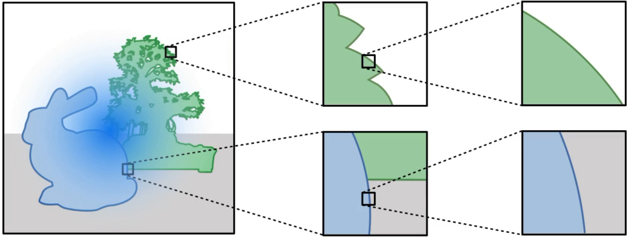
Figure 27.
For integrands with small angular support, visibility discontinuities typically consist of a single object silhouette.
A typical shading integral can contain complex parameter-dependent discontinuities. However, when the integrand has small angular support (e.g., narrow pixel reconstruction filters, glossy BSDF lobes, or small light sources), the discontinuity within the support reduces to the silhouette of a single object, as shown in Fig. .
The displacement of a silhouette on $S^2$ under infinitesimal perturbations of $\pi$ is well approximated by a spherical rotation (the spherical counterpart of a planar domain translation). As the support shrinks, this approximation improves, becoming exact in the limit. Assuming a suitable rotation $R(\omega, \pi)$ exists, the change of variables
makes $f(R(\omega, \pi), \pi)$ continuous with respect to $\pi$ for each direction $\omega$. The rotation determinant is $|\operatorname{det} J_R| = 1$, and $R$ depends explicitly on $\pi$.
Figure 28.
Zooming into the support of a convolution shows how small-support kernels isolate single geometric edges, making local rotations a good approximation.
Rotations are simple to compute and accurately track local boundary movements. Using $R$ to reparameterize the integral yields the Monte Carlo estimator:
$$
E = \frac{1}{N} \sum_{i=1}^N \frac{f(R(\omega_i, \pi), \pi)}{p(\omega_i, \pi_0)} \approx I
$$
where $\omega_i \sim p(\cdot, \pi_0)$ are drawn from the default sampling distribution (e.g., BSDF sampling) evaluated at $\pi_0$ rather than $\pi$, removing sample dependency on $\pi$.
Figure 29.
Spherical rotations (left) approximate silhouette motion, while spherical convolution (right) reduces large-support integrands to narrow kernels.
When integrands have large support on $S^2$, they contain multiple interacting silhouettes that violate the single-object assumption, causing bias in local rotation estimates.
To resolve this, we leverage the property that the integral of a function $f$ equals the integral of its spherical convolution:
By choosing $k$ to be a smooth, concentrated distribution (such as a von Mises-Fisher distribution) with small angular support, the inner integral is restricted to a small domain, restoring compatibility with local rotations.
To evaluate Equation $\eqref{eq:reparam_conv}$ numerically, we sample outer directions $\omega_i$ and offset directions $\mu_i \sim k(\cdot, \omega_i)$, giving the combined estimator:
$$
I \approx E = \frac{1}{N} \sum_{i=1}^N
\frac{f(R_i(\mu_i,\pi),\pi)\,
k(R_i(\mu_i,\pi),\omega_i(\pi),\pi)}
{p(\omega_i(\pi),\pi)\,p_k(\mu_i)}
$$
This is the parameter dependence shown in the paper’s Equation 18: the outer proposal $p$ and convolution kernel $k$ are evaluated consistently at their transformed, parameter-dependent arguments. Kernel width provides a trade-off between variance and bias: narrower kernels model local edge displacements accurately but decrease the chance of finding discontinuities (increasing variance), while wider kernels reduce variance but increase rotation-approximation bias. For a fixed kernel, the practical estimator is not consistent: tracing more paths reduces variance but does not remove bias from an imperfect rotation or a missed discontinuity.
Determining rotation matrices that track boundary motion without explicitly searching for silhouette edges is key to making this reparameterization practical for high scene complexity.
A central insight of Loubet et al. is that finding a suitable change of variables does not require identifying silhouette edges or even knowing whether an integrand contains a discontinuity. The only required information is how surface points move under infinitesimal perturbations of scene parameters $\pi$.
Because the integrand has small support, the displacement of points on silhouette edges closely approximates the displacement of other nearby surface positions on the same object. We exploit this by tracing a small batch of auxiliary rays within the integrand’s support (this number has an impact on the probability of missing a discontinuity by sampling only one of the objects of the integrand,
which results in bias). Using distance and surface normal information, a heuristic selects a candidate occluder point whose motion under parameter changes tracks that of the silhouette.
Projecting the selected point onto $S^2$ gives direction $\omega_P(\pi)$, with $\omega_{P_0} = \omega_P(\pi_0)$. A differentiable rotation matrix $R(\pi)$ is then constructed to satisfy:
Thus $R(\pi_0) = I$ (leaving primal ray tracing unchanged) while its derivative tracks the occluder’s motion to first order. Appendix B of Loubet et al. provides a closed-form formula for $R(\pi)$.
Figure 30.
Overview of the reparameterization algorithm. For each integral, a small number of rays are intersected against the scene geometry (steps 1, 3, 5) and the resulting information is used to construct suitable local rotations (red arcs). These rotations do not affect the primal computation (steps 2, 4, 6) but introduce gradients that correct for the presence of discontinuities.
Crucially, this construction requires only standard ray intersection queries (well suited for hardware acceleration) and the auxiliary rays can often be reused for Monte Carlo integration.
A naive implementation of the change-of-variables estimator introduced above exhibits significant gradient variance. Loubet et al. resolve this by leveraging control variates constructed from correlated path pairs.
At $\pi = \pi_0$, the transformation is the identity $\mathcal{T}(y, \pi_0) = y$, giving $w_i(\pi_0) = 1$. The primal estimate $E = \frac{1}{N}\sum f(y_i, \pi_0)$ is unaffected.
Differentiating $E$ with respect to $\pi$ via the product rule yields:
While the expected derivative of the weights $w_i(\pi)$ is zero for any distribution $k$, individual sample weight gradients $\frac{\partial w_i(\pi)}{\partial \pi}$ are non-zero and fluctuate randomly. These fluctuations introduce severe variance into gradient estimates.
The classical control variates method reduces the variance of an estimator $E$ using a correlated estimator $F$ with known expectation $\mathbb{E}[F]$:
$$
E' = E + \alpha (F - \mathbb{E}[F])
$$
where optimal variance reduction is achieved when $\alpha = -\frac{\operatorname{Cov}(E, F)}{\operatorname{Var}(F)}$.
Since $\mathbb{E}\left[ \frac{\partial w_i(\pi)}{\partial \pi} \right] = 0$, we construct a zero-expectation control variate $F(\pi) = \frac{1}{N}\sum_{i=1}^N w_i(\pi)$, with $\mathbb{E}[F(\pi_0)] = 1$. This modifies the estimator to:
If $f(x) = c$ is constant, setting $\alpha = -c$ makes $\frac{\partial E'}{\partial \pi} = 0$ for every sample point, completely eliminating gradient variance. For a general smooth function, $\alpha$ should therefore approximate the negative average value of $f$. It may reduce variance substantially without introducing bias, provided it is independent of the weight gradient to which it is applied.
To determine $\alpha$ without introducing bias (as $\alpha$ must remain independent of sample weights $w_i$), Loubet et al. employ a cross-weighting scheme using pairs of correlated paths ($r_0$ and $r_1$).
where $W_{i,l}(\pi)$ is the product of reparameterization weights along path $i$ up to bounce $l$, and $f_{i,l}(\pi)$ represents throughput and emitter radiance.
By using $\alpha=-f_{1,l}$ for path 0 and $\alpha=-f_{0,l}$ for path 1, the cross-reduced path contribution $r'$ is:
Correlated path pairs reuse the random numbers for path-construction steps except those that affect the local reparameterization weights. Those samples remain independent so that $f_{0,l}$ is uncorrelated with $\partial_\pi W_{1,l}$ and vice versa. Under this independence condition, cross-reduction lowers gradient variance for direct and multi-bounce illumination without adding bias, at the cost of tracing paired paths.
Unbiased Warped-Area Sampling (Bangaru et al., 2020)#
Bangaru et al. [8] ask whether the boundary term can be estimated using the same area samples as an ordinary path tracer. Their answer is yes: apply the divergence theorem to replace flux through visibility boundaries by divergence throughout the smooth interior. The resulting method does not enumerate or sample silhouette edges. This is different from merely smoothing visibility; the construction specifies conditions under which the area estimator represents the exact boundary derivative.
Figure 31.
Taxonomy of differentiable rendering techniques categorizing edge sampling, reparameterization, and warped-area methods.
Let $D$ be an angular integration domain and partition it, only for the derivation, into disjoint regions $D_i(\boldsymbol{\pi})$ such that $f(\boldsymbol{\omega};\boldsymbol{\pi})$ is smooth inside each region and all jumps lie on their boundaries. Reynolds transport theorem gives
where $D_i'=D_i\setminus\partial D_i$. The first term is the usual interior derivative. The second measures the flux produced by moving discontinuities.
This partition is only a device used in the proof; evaluating the estimator does not require clipping the scene into the regions $D_i$ or enumerating their boundaries.
Introduce a vector field $\mathbf{V}_{\boldsymbol{\pi}}(\boldsymbol{\omega})$ that interpolates the boundary velocity into the interior. Applying the divergence theorem to $f\mathbf{V}_{\boldsymbol{\pi}}$ rewrites the boundary contribution as:
Consequently, an area sample contributes three conceptually different derivatives:
$$
\partial_{\boldsymbol{\pi}} f + \partial_{\boldsymbol{\omega}}f\cdot\mathbf{V}_{\boldsymbol{\pi}} + f\,\nabla_{\boldsymbol{\omega}}\!\cdot\mathbf{V}_{\boldsymbol{\pi}}.
$$
The first is the ordinary interior derivative. The second moves the sample with the warp. The third accounts for local expansion or contraction of the warped domain. Dropping the divergence term is only valid for volume-preserving warps.
The divergence-theorem argument requires the warp field to satisfy two conditions:
Interior continuity: $\mathbf{V}_{\boldsymbol{\pi}}$ is $C^0$ in $D'=D\setminus\partial D$.
Boundary consistency: as $\boldsymbol{\omega}$ approaches a boundary point $\boldsymbol{\omega}_b$, $\mathbf{V}_{\boldsymbol{\pi}}(\boldsymbol{\omega})$ approaches the true boundary velocity $\partial_{\boldsymbol{\pi}}\boldsymbol{\omega}_b$.
The equality is required as a limit from the smooth regions; the field need not be defined on the measure-zero boundary itself. These conditions are the central correctness criterion of the paper. A smooth field with the wrong boundary value remains biased, and a field that is correct at a silhouette but discontinuous in the interior cannot be inserted into the area formula above.
Differentiating the intersection gives $\partial_{\boldsymbol{\pi}}\mathbf{y}$ and $\partial_{\boldsymbol{\omega}}\mathbf{y}$. The paper’s direct warp is the angular motion whose projection produces the surface motion:
This matrix form incorporates the correction in the paper’s 2022 erratum: the denominator is not a Jacobian determinant. The equation is a Jacobian solve, with matrix-valued numerator and denominator when the quantities are multidimensional.
The direct warp has the correct limiting motion on a silhouette, but it jumps when neighboring directions hit different surfaces. Bangaru et al. therefore filter it using a normalized, boundary-aware harmonic convolution:
$D$ is a smooth angular distance, such as one induced by a von Mises-Fisher kernel ($D(\boldsymbol{\omega},\boldsymbol{\omega}') = e^{\kappa(1-\langle\boldsymbol{\omega},\boldsymbol{\omega}'\rangle)} - 1$). $B$ is a boundary test: a non-negative scalar function that approaches zero at any visibility boundary ($B(\boldsymbol{\omega}') \to 0$ as $\boldsymbol{\omega}' \to \partial \Omega$). Crucially, evaluating $B$ is far cheaper than searching for silhouette edges explicitly.
For triangle meshes, Bangaru et al. construct $B$ at each mesh vertex $v$ using the dot product between the ray direction $\boldsymbol{\omega}'$ and the vertex normal $\mathbf{n}$:
where $\beta = 0.01$ controls the spread rate. At a silhouette point, the ray direction is perpendicular to the normal ($\langle\boldsymbol{\omega}', \mathbf{n}\rangle = 0$), forcing $\mathcal{B}_v = 0$. Vertex values $\mathcal{B}_v$ are then interpolated across triangle faces via barycentric coordinates. Because the harmonic weight becomes singular ($w \to \infty$) near a boundary, the normalized convolution collapses to the direct warp there. It therefore preserves boundary consistency while smoothing the field in the interior.
Hence the filtered warp approaches the boundary-consistent direct warp as the primary direction approaches a silhouette. The field may remain undefined exactly on the silhouette, where the harmonic weights become infinite, because the area estimator only evaluates the smooth interior.
This establishes a local relationship between reparameterization and the warp-field formulation, but it does not imply that every chosen reparameterization is exact. A spherical rotation has unit Jacobian and therefore produces a divergence-free field. Some boundary motions require nonzero divergence, so a rotation cannot satisfy the boundary conditions in general. Bangaru et al. interpret the approximations of Loubet et al. as producing a field that can be smooth without being boundary-consistent, which explains the remaining bias. Warped-area sampling instead makes continuity and boundary consistency explicit and uses the harmonic construction to satisfy both without enumerating silhouettes.
Appendix C proves both directions of this relationship. A transformation $\mathcal{T}$ induces the field above by differentiating at the evaluation point $\boldsymbol{\pi}_0$. Conversely, one possible Euclidean transformation generated by a given field is
The construction is not unique; on the sphere, the appendix also gives a rotational solution. This equivalence concerns the infinitesimal field induced by a transformation. Unbiasedness still depends on whether that field is continuous and has the correct limiting boundary velocity.
At each ordinary path-tracing direction $\boldsymbol{\omega}$, the algorithm:
traces the primary ray and recursively evaluates radiance $L$, its parameter derivative $\partial_{\boldsymbol{\pi}} L$, and directional derivative $\partial_{\boldsymbol{\omega}}L$;
samples auxiliary directions $\boldsymbol{\omega}'_i$ around $\boldsymbol{\omega}$ from a von Mises-Fisher distribution;
differentiates each auxiliary ray intersection, evaluates $B_i$, and forms importance-corrected harmonic weights $w_i$;
estimates both $\widehat{\mathbf{V}}_{\boldsymbol{\pi}}$ and $\nabla_{\boldsymbol{\omega}}\cdot\widehat{\mathbf{V}}_{\boldsymbol{\pi}}$ from the weighted samples; and
to the ordinary interior derivative $\partial_{\boldsymbol{\pi}} L$.
There is an important qualification in the paper’s title. With a fixed number $N'$ of auxiliary rays, replacing both integrals in the normalized convolution by sample averages creates a ratio estimator. Since $\mathbb E[1/Z]\neq1/\mathbb E[Z]$, this finite-$N'$ version is consistent but not unbiased. It converges to the exact warp as $N'\to\infty$.
The provably unbiased variant applies Russian-roulette debiasing to the convergent sequence of normalization estimates. If $T_0,T_1,\ldots$ converges to $T$, write
$$
T=T_0+\sum_{i=1}^{\infty}(T_i-T_{i-1})
$$
and randomly truncate this telescoping series using a geometric distribution, dividing each retained difference by its survival probability. This makes the warp estimate, and hence the derivative estimate, unbiased, at the cost of a random amount of work.
The raw area estimator has substantial variance even in smooth regions. Auxiliary directions are paired antithetically by rotating them $180^\circ$ around the kernel center, making the derivatives of symmetric weights negatively correlated. A locally linear approximation of the warp is then used as a control variate. These operations reduce variance without changing the expectation and are separate from the Russian-roulette construction that establishes unbiasedness.
The paper is explicit about where its unbiasedness guarantee does and does not apply:
Implicit Edges: The triangle-mesh boundary test $\mathcal{B}$ relies on face normals and open/silhouette edges. It does not automatically detect implicit edges created by triangle self-intersections, where geometric boundaries do not coincide with mesh edges. Near such intersections, $\mathcal{B}$ fails to vanish, causing the convolution to average neighboring warps rather than applying singular weights. While the result remains visually accurate and behaves similarly to Loubet et al., the field loses its strict boundary consistency guarantee and is no longer provably unbiased.
Unbounded Work: The Russian-roulette estimator has theoretically unbounded work and storage. Any deterministic cap on the number of auxiliary rays reintroduces truncation bias.
Domain Extensions: The divergence argument extends in principle to motion blur and depth of field by enlarging the integration domain and redefining $B$. Extension to path space is less immediate because one path-space point can cross several occluders, so the correct boundary definition remains unresolved in this paper.
Universal Boundary Test: The method augments a unidirectional path tracer and naturally supports secondary transport, but the paper does not claim that its particular triangle boundary test is universal. Other geometry representations (e.g. SDFs, Bezier curves) require their own test satisfying the same limiting condition.
The continuity argument can be made directly from the normalized convolution. Writing $Z(\boldsymbol{\omega})=\int w(\boldsymbol{\omega},\boldsymbol{\omega}')\,\mathrm d\boldsymbol{\omega}'$, the quotient rule gives
Only the derivative of $w$ with respect to the primary direction appears. Therefore $B(\boldsymbol{\omega}')$ itself need not be differentiable or even continuous across visibility boundaries: a differentiable distance function $D(\boldsymbol{\omega},\boldsymbol{\omega}')$ is sufficient to keep the divergence finite at interior points.
A discontinuous pixel filter (such as a box filter) introduces another moving boundary at the edge of its support. To ensure the divergence theorem holds across pixel boundaries without requiring a dedicated pixel boundary test, Bangaru et al. enforce a continuous pixel prefilter using a truncated Gaussian filter (truncated at a radius of $4\sigma$, where kernel values drop below floating-point precision).
Given the mathematical tools described above, we will discuss the differentiation of the rendering equation (RE) with respect to arbitrary scene parameters.
Physically-based rendering of surfaces has been a central topic in computer graphics for decades and is governed by the well-known rendering equation (RE). The RE is an integral equation stating that the (steady-state) radiance $L$ at any surface point $\mathbf{x}$ with direction $\boldsymbol{\omega}_o$ is given by:
where $L_i$ is the incident radiance, $\mathrm{d}\sigma$ is the solid-angle measure, and $f_s$ denotes the BSDF multiplied by the cosine factor $|\mathbf{n}\cdot\boldsymbol{\omega}_i|$. We use a BSDF rather than a reflection-only BRDF because general scenes can include both reflection and transmission, for example at refractive interfaces. Light directions are written as bold unit vectors (e.g., $\boldsymbol{\omega}_i, \boldsymbol{\omega}_o$).
The RE has no analytical solution in general, and numerous numerical methods have been developed. Some of the widely adopted examples include unbiased methods like unidirectional and bidirectional path tracing, as well as biased ones such as photon mapping and lightcuts.
Before differentiating the full RE $\eqref{eq:rendering-equation}$, we will first consider the case of direct illumination as a warm-up. Specifically, the radiance $L_r$ resulting from exactly one reflection at a surface point $\mathbf{x}$ with direction $\boldsymbol{\omega}_o$ equals
where $\mathbf{y}$ represents the closest intersection of a light ray originating at $\mathbf{x}$ with direction $\boldsymbol{\omega}_i$, i.e., $\mathbf{y} = \operatorname{rayTrace}(\mathbf{x}, \boldsymbol{\omega}_i)$. Unlike RE $\eqref{eq:rendering-equation}$, which takes the form of an integral equation, Eq. $\eqref{eq:direct-illumination}$ is a simple spherical integral as its right-hand side involves only known quantities.
We now consider the problem of calculating the derivative of $L_r(\mathbf{x}, \boldsymbol{\omega}_o)$ with respect to some abstract scene parameter $\pi \in \mathbb{R}$. Given $\mathbf{x}$ and $\boldsymbol{\omega}_o$, let $f_{direct}(\boldsymbol{\omega}_i; \mathbf{x}, \boldsymbol{\omega}_o) := L_e(\mathbf{y}, -\boldsymbol{\omega}_i) \; f_s(\mathbf{x}, \boldsymbol{\omega}_i, \boldsymbol{\omega}_o)$. It holds that
where $\mathrm{d}\ell$ is the curve-length measure. This is exactly the RTT split from before, specialized to a spherical integral: the interior term integrates over the ($\pi$-independent) sphere $\mathbb{S}^2$, and the boundary term picks up the jump of $f_{\text{direct}}$ across the 1D discontinuity curves $\Delta \mathbb{S}^2$, the silhouette-induced jumps in $L_e$, as they move with $\pi$. For any $\boldsymbol{\omega}_i \in \mathbb{S}^2$, $\mathbf{n}^{\perp}(\boldsymbol{\omega}_i)$ is, as before, the tangent-space vector at $\boldsymbol{\omega}_i$ perpendicular to the discontinuity curve.
Figure 32.
The normal directions of arcs and circles (that are respectively the projections of line segments and spheres) as spherical curves.
Assuming the (cosine-weighted) BSDF $f_s(\mathbf{x}, \boldsymbol{\omega}_i, \boldsymbol{\omega}_o)$ to be continuous with respect to $\boldsymbol{\omega}_i$, which is usually the case except for perfectly specular BSDFs, the discontinuities of the integrand $f_{direct}$ fully emerge from those of incident emission $L_e(\mathbf{y}, \boldsymbol{\omega}_i)$, which is generally discontinuous due to occlusions. Therefore,
Based on the analysis above, we now differentiate the full rendering equation (RE) $\eqref{eq:rendering-equation}$ using the Reynolds transport theorem ($\eqref{eq:reynolds-transport-theorem}$). This yields another integral equation, which we call the differential rendering equation.
We begin by applying the derivative operator $\partial_\pi$ to both sides of the standard rendering equation:
Since the scene geometry may move as the parameter $\pi$ changes, the integration domain inherently contains moving boundaries (i.e., silhouettes). Applying the Reynolds Transport Theorem ($\eqref{eq:reynolds-transport-theorem}$) splits the derivative of this integral into an interior and a boundary component:
Note on the boundary term: Notice that we wrote the jump of the integrand as $f_s \Delta L_i$ rather than $\Delta(L_i f_s)$. This assumes that the cosine-weighted BSDF $f_s$ evaluates smoothly and continuously with respect to the incoming direction $\boldsymbol{\omega}_i$. For typical materials such as diffuse and rough microfacet models, this holds: the discontinuity is caused by the incoming radiance $L_i$ abruptly jumping when an integration ray sweeps past a silhouette edge or shadow boundary. The notable exception is perfectly specular materials, whose BSDFs are Dirac delta functions; handling those requires a different mathematical approach, such as attached sampling.
Inside the interior integral, we expand the derivative of the product $\partial_\pi (L_i f_s)$ using the standard product rule:
Substituting this expansion back into the equation allows us to regroup the terms into two distinct transport components. We collect the terms acting as “sources” of differential radiance into one group, and the term representing scattered differential radiance into another:
This final equation shares the exact same structure as the original rendering equation. Instead of standard light emission and scattering, it describes the emission and scattering of differential radiance (gradients).
The differential emission term $Q(\mathbf{x}, \boldsymbol{\omega}_o)$ acts as the source of gradients. It evaluates to a non-zero value at any point where the primary emission changes ($\partial_\pi L_e$), the material scattering properties change ($\partial_\pi f_s$), or a silhouette edge moves to uncover a different object ($f_s \Delta L_i$). During Monte Carlo integration, we compute this local change $Q$ at every path vertex and add it to the running gradient estimate.
The differential scattering term $\int (\partial_\pi L_i) f_s \mathrm{d}\sigma$ handles the propagation of these gradients. Here, $\partial_\pi L_i$ represents the derivative of the incident radiance arriving from the previous bounce. Just like standard radiance, this incoming differential radiance is multiplied by the material’s BSDF ($f_s$) and scattered towards the camera.
Consequently, when a Monte Carlo path tracer simulates this process, it unrolls the recursion identical to forward rendering. For a light path with vertices $x_1 \to x_2 \to x_3 \to \text{Camera}$, the total gradient expands mathematically via the chain rule as:
In practice, this means we trace a standard light path and, at each bounce, compute the local differential emission $Q$, add it to the accumulated gradient, and multiply the running total by the surface BSDF as the path continues.
Nimier-David et al. [7] begin from the same differential rendering equation derived above, but reorganize reverse-mode differentiation as a second physical transport simulation. The objective is not a Jacobian image for one parameter. It is the vector-Jacobian product required by optimization: the derivative of one scalar objective with respect to all active scene parameters.
Write the ordinary renderer as $\mathbf y=f(\boldsymbol{\pi})$ and the scalar objective as $g(\mathbf y)$. Radiative backpropagation separates one optimization iteration into:
an ordinary, non-differentiable render $\mathbf y=f(\boldsymbol{\pi})$;
differentiation of the comparatively small image-space objective, producing the adjoint rendering
$$
\delta\mathbf y=J_g(\mathbf y)^T;
$$
a radiative-backpropagation simulation estimating
$$
\delta\boldsymbol{\pi}=J_f(\boldsymbol{\pi})^T\delta\mathbf y.
$$
$\delta\mathbf y$ says how each rendered pixel should change to reduce the objective. The sensor emits this quantity into the scene as adjoint radiance. Scattering transports it to emitters, materials, and media whose local derivatives contribute to $\delta\boldsymbol{\pi}$.
In pseudocode:
defgrad(x):# 1. Ordinary rendering (no AD)y=f(x)# 2. Differentiate objective at y (manually or w/ AD)δ_y=J_gᵀ(y)# 3. Estimate δ_x = J_fᵀ δ_y using radiative backpropagationreturnradiative_backprop(x,δ_y)
Figure 33.
Overview of Radiative Backpropagation: Differentiation separates into (1) a fast primal rendering step, (2) objective differentiation yielding adjoint rendering $\delta_\mathbf{y}$, and (3) an adjoint light transport simulation emitting $\delta_\mathbf{y}$ from the sensor to accumulate parameter gradients $\delta_\boldsymbol{\pi}$.
Note on Static Visibility Boundaries: In the original Radiative Backpropagation formulation (Nimier-David et al., 2020), differentiation is derived assuming static geometry (fixed visibility boundaries). Because fixed scene geometry does not move as parameter $\pi$ changes ($\partial_\pi \boldsymbol{\omega}_i = \mathbf{0}$), the boundary movement velocity is zero and the Boundary Integral vanishes ($\mathbf{=0}$), reducing the differential transport equation to Direct Emission, Diff. Scattering, and Material Emission.
Grouping the non-scattering gradient source terms into the Differential Emission term $Q(\mathbf{x}, \boldsymbol{\omega}_o)$:
To analyze reverse-mode backpropagation abstractly, we express differential light transport using linear operators:
Ray Transport Operator $\mathcal{G}$: Maps outgoing differential radiance at the closest surface hit $\mathbf{y} = r(\mathbf{x}, \boldsymbol{\omega}_i)$ to incident differential radiance at $\mathbf{x}$:
Substituting $\partial_\pi L_i = \mathcal{G} \partial_\pi L_o$ into the differential scattering term allows us to write the entire differential rendering equation in compact operator form:
where $\mathcal{S} = (\mathcal{I} - \mathcal{K}\mathcal{G})^{-1} = \sum_{k=0}^\infty (\mathcal{K}\mathcal{G})^k$ is the full path-scattering solution operator.
If $A_e$ is the emitted adjoint radiance obtained by back-projecting the loss gradient $\delta\mathbf{y} = \mathbf{J}_g^T(\mathbf{y})$ from the sensor into the scene, the desired vector-Jacobian product for parameter optimization is the inner product:
For reciprocal, energy-conserving transport under the ray-space measure, the transport operators $\mathcal{G}$, $\mathcal{K}$, and $\mathcal{S}$ are self-adjoint ($\mathcal{G}^* = \mathcal{G}, \mathcal{S}^* = \mathcal{S}$). Transferring the operators to the left side of the inner product yields:
where $A = \mathcal{G}\mathcal{S} A_e$ is the incident adjoint radiance field. This duality is the central realization of Radiative Backpropagation: rather than transporting a high-dimensional vector field of parameter derivatives $Q$ forward, we simulate a scalar adjoint path tracing pass from the camera to compute $A$, and evaluate its inner product with local differential sources $Q$ whenever a path hits a differentiable object or boundary.
This is the central step: rather than transport the enormous vector-valued field $Q$, transport the scalar adjoint field from the sensor and evaluate its inner product with sparse local derivatives when a path reaches a differentiable object.
The corresponding incident and outgoing adjoint radiance satisfy
$$
A_i=\mathcal G A_o,
\qquad
A_o=A_e+\mathcal K A_i.
$$
The paper obtains $A_e$ directly from the adjoint image. If $W_k(\mathbf{x},\boldsymbol{\omega}_o)$ is pixel $k$’s sensor importance and $\delta y_k$ is that pixel’s objective derivative, then
which turns the discrete sum over pixel derivatives into the ray-space inner product $\langle A_e,\partial_{\boldsymbol{\pi}}L_i\rangle$. For a pinhole camera, $A_e$ can be viewed as a textured projector that emits the adjoint image into the scene.
These equations can be sampled by an ordinary path-tracing random walk launched from the sensor. At a surface hit, the algorithm:
backpropagates the current adjoint weight through $L_e$ into active emitter parameters;
samples a BSDF direction $\boldsymbol{\omega}_i$;
backpropagates the weight $A_i L_i/p(\boldsymbol{\omega}_i)$ through the sampled BSDF value into active material parameters; and
continues the adjoint path with throughput $f_s/p$.
The local reverse-mode operation is sparse. A texture lookup, for example, contributes only to nearby texels rather than constructing a dense derivative with respect to every scene parameter.
defradiative_backprop(π,δ_y):# Initialize parameter gradient(s) to zeroδ_π=0for_inrange(num_samples):# Importance sample a ray from the sensorx,ω_o,weight=sensor.sample_ray()# Evaluate the adjoint emitted radianceweight*=A_e(δ_y,x,ω_o)/num_samples# Propagate adjoint radiance into the sceneδ_π+=radiative_backprop_sample(π,x,ω_o,weight)# Finished, return gradientsreturnδ_πdefradiative_backprop_sample(π,x,ω_o,weight):# Find an intersection with the scene geometryy=r(x,ω_o)# Backpropagate to parameters of emitter, if anyδ_π=adjoint([[L_e(y,-ω_o)]],weight)# Sample a ray from the BSDFω_i,bsdf_value,bsdf_pdf=sample_f_s(y,-ω_o,·)# Backpropagate to parameters of BSDF, if anyδ_π+=adjoint([[f_s(y,-ω_o,ω_i)]],weight*L_i(y,ω_i)/bsdf_pdf)# Recursereturnδ_π+radiative_backprop_sample(π,y,ω_i,weight*bsdf_value/bsdf_pdf)
The paper does not claim that camera-path sampling is the only estimator. It points out that $Q$ may have large components at specific differentiable objects, suggesting connection strategies analogous to next-event estimation. If many of those connections are occluded, scattering them before connection leads to a family of bidirectional strategies. Casting reverse differentiation as transport is useful precisely because ordinary rendering tools such as importance sampling, next-event estimation, and bidirectional connection strategies become available.
The derivation and prototype make several explicit assumptions:
Static Sensor Importance: Sensor importance $W_k$ is treated as static. A differentiable camera would contribute an additional local derivative term.
Self-Adjoint Operators: Surface operators are self-adjoint under reciprocal, energy-conserving BSDFs and the ray-space measure. Nonreciprocal transport (e.g. non-reciprocal BSDFs or camera lenses) would require true adjoint operators rather than reusing primal ones.
Volumetric Extension: The same adjoint construction extends directly to participating media by replacing surface transport operators with their volumetric counterparts (RBP paper, Appendix A.1).
Visibility Derivatives (Edge Sampling vs. Reparameterization):
Edge Sampling (Li et al., 2018) [10]: Explicitly samples silhouette edges, which requires modifying the theoretical formulation to add extra 1D boundary integral terms to the differential emission source $Q$.
Reparameterization / Change of Variables (Loubet et al., 2019) [11]: Performs a parameter-dependent coordinate warp so that discontinuities remain static under scene perturbations ($\partial_{\boldsymbol{\pi}}\boldsymbol{\omega}_i = \mathbf{0}$). This allows RBP to compute visibility-aware gradients without changing any of the adjoint derivations.
At an intersection $\mathbf{y} = r(\mathbf{x}, \boldsymbol{\omega}_o)$, an adjoint path contributes two local VJPs corresponding to the terms of $Q$:
The path then continues with adjoint throughput multiplied by $f_s/p$. This is the Monte Carlo realization of $\langle\mathcal G\mathcal S A_e,Q\rangle$, not a reversal of stored primal vertices.
A key practical bottleneck is that the differential emission term $Q$ depends on the unknown primal incident radiance $L_i$. Evaluating $Q$ at every differentiable interaction requires launching a recursive primal path-tracing query. Along a path of depth $D$ with differentiable surfaces at each bounce, these suffix queries have lengths $D, D-1, \ldots, 1$, leading to quadratic time complexity $\mathcal{O}(D^2)$ (a bottleneck also reported by Zhang et al. (2019)[16] for forward AD). Non-differentiated interactions do not trigger this extra work.
To mitigate this quadratic overhead in long light paths, one can precompute an approximate spatio-directional data structure during the primal phase (such as a Path Guiding tree [Müller et al., 2017] [17]) to perform fast $\mathcal{O}(1)$ interpolant queries of $L_i$ during adjoint backpropagation.
Thus, RBP solves the reverse-mode storage and transport problem; it is not by itself a solution to moving visibility discontinuities unless paired with reparameterization or boundary sampling.
Figure 34.
Illustration of the quadratic $\mathcal{O}(D^2)$ complexity in Radiative Backpropagation. An adjoint path launched from the camera (black rays) evaluates local parameter derivatives ($\frac{\partial f_s}{\partial \boldsymbol{\pi}}$, $\frac{\partial L_e}{\partial \boldsymbol{\pi}}$) at each differentiable surface hit (red dots). To estimate the unknown primal incident radiance $L_i$ in $Q$, a recursive primal path-tracing query (gray rays) is launched at every bounce.
Biased I: replace $L_i$ in $Q$ by $1$. This removes recursive radiance queries and reduces time to $O(D)$, but changes the gradient.
Biased II: pipeline optimization by using the previous iteration’s adjoint rendering with the current iteration’s rendering Jacobian. This overlaps primal and adjoint work but introduces an intentional one-iteration mismatch.
The RBP paper originally claimed that Biased I preserves gradient signs. Its published erratum withdraws this claim, and Vicini et al. [15] give an explicit counterexample: each local product preserves its sign when multiplied by positive radiance, but globally summing many differently weighted signed contributions need not preserve the sign. Biased I can still work well and often reduces variance, but it must be described as a heuristic rather than a directionally correct gradient estimator.
For Biased II, if superscripts denote optimization iterations, the propagated quantity is
instead of using $\delta\mathbf y^{(i)}$. It is reasonable only when the rendering Jacobian and objective gradient vary slowly between iterations. The paper labels the combined approximation Biased I + II.
The unbiased algorithm is constant-memory with respect to path length, but its repeated $L_i$ queries make time quadratic. This is prohibitive for highly scattering media with thousands of events. Biased I reduces that cost to linear time but is not a correct derivative. The formulation above omits moving-visibility derivatives and does not handle derivatives through ideal specular BSDF sampling. Faster gradient evaluation also does not remove nonconvexity or poor conditioning from the inverse problem itself.
Radiative backpropagation obtains constant memory by recomputing a fresh primal suffix at each differentiable interaction, causing the quadratic cost above. Vicini et al. [15] instead replay the same complete random walk and reconstruct all required suffix radiances incrementally. Under the sampling and discontinuity assumptions below, Path Replay Backpropagation (PRB) is unbiased, uses memory independent of path length, and takes time linear in the number of scattering events.
Figure 35.
Illustration of linear $\mathcal{O}(D)$ complexity in Path Replay Backpropagation (PRB). Rather than spawning branching quadratic primal suffix trees, PRB replays the exact same random walk (green rays) alongside the adjoint path (black rays). Local parameter derivatives ($\frac{\partial f_s}{\partial \boldsymbol{\pi}}$, $\frac{\partial L_e}{\partial \boldsymbol{\pi}}$) are evaluated at each surface hit (red dots) in linear time and constant memory.
First consider a detached sampling strategy: random samples and sampled directions are constant with respect to $\boldsymbol{\pi}$, emitters are static, and parameter-dependent discontinuities are absent or handled separately. For a path with vertices $0,\ldots,N$, let
with $L_0 = 0$ and $\beta_0 = 1$. The forward evaluation retains only the final accumulated radiance $L_N$. A second evaluation starts from the same random state and therefore visits the exact same vertices in the same camera-to-light order.
where $\widehat L_{i,k}$ is the radiance contributed by the rest of this particular sampled path, expressed relative to the throughput after vertex $k$. Since $\beta_k = \beta_{k-1} f_{s,k} / p_k$,
which is exactly the Monte Carlo weight for the $L_i\,\partial_{\boldsymbol{\pi}}f_s$ term in the differential rendering equation. Repeating the subtraction updates $R_k$ in constant time, so all suffix-radiance factors are recovered in one replay rather than by $N$ recursive suffix queries.
Both evaluations traverse the path forward; PRB neither stores and reverses path vertices nor checkpoints the full computation. Given the same random stream, its derivative agrees with conventional reverse-mode AD sample-for-sample, apart from floating-point evaluation order. If the image-space loss derivative is itself estimated from a noisy primal image, that primal estimate must be statistically independent of the correlated replay pair to avoid bias.
The subtraction may lose precision when one vertex dominates the complete path contribution. This is the same regime in which the primal radiance sum is already close to floating-point accuracy limits.
Detached differentiation cannot optimize parameters that move ideal specular samples, such as the index of refraction, geometry, or normals of smooth dielectrics and conductors. To include these dependencies, write inverse-transform sampling as a parameter-dependent map $\mathbf{x} = T(\mathbf{u}, \boldsymbol{\pi})$ from $\mathbf{u} \in [0,1]^n$ to path space. The reparameterized pixel integral is
A perturbation at one interaction therefore changes all later vertices and their BSDF and emission factors. PRB reconstructs this non-local dependence using the differential relationship between adjacent path segments. A ray can be represented by two local surface coordinates at its origin and two at its endpoint, reducing the Jacobian between adjacent segments to a $4\times4$ matrix. Explicitly propagating these small ray, throughput, and radiance Jacobians carries all derivative information between interactions without storing a path-length AD graph. A position-position parameterization keeps the matrix entries dimensionally compatible and is better conditioned than mixing positions and angles.
# Pass 1: Primal path tracing pass (Attached)defsample_path(ray):L=0;β=1J_L=0_3,4;J_β=0_3,4;J_ray=I_4foriinrange(N):L+=β*L_e(...)ω_i,bsdf_value,bsdf_pdf=sample_bsdf(...)bsdf_weight=bsdf_value/bsdf_pdfray_prime=spawn_ray(ω_i,...)# Compute the directional radiance derivativeJ_ray_prime,J_bsdf,J_L_e=forward_grad(ray,{ray_prime,bsdf_weight,L_e})J_bsdf=J_bsdf@J_rayJ_L_e=J_L_e@J_rayJ_ray=J_ray_prime@J_rayJ_L+=β*J_L_e+L_e*J_βJ_β=bsdf_weight*J_β+β*J_bsdfβ*=bsdf_weightreturnL,J_L# Pass 2: Adjoint replay pass (Attached)defsample_path_adjoint(ray,L,J_L,δL):β=1;J_ray=I_4;δ_π=0foriinrange(N):L-=β*L_e(...)ω_i,bsdf_value,bsdf_pdf=sample_bsdf(...)bsdf_weight=bsdf_value/bsdf_pdfray_prime=spawn_ray(ω_i,...)J_ray_prime,J_bsdf,J_L_e=forward_grad(ray,{ray_prime,bsdf_weight,L_e})J_bsdf=J_bsdf@J_rayJ_L_e=J_L_e@J_rayJ_ray=J_ray_prime@J_ray# Update the directional radiance derivativeJ_L-=L/bsdf_value*J_bsdf+β*J_L_eJ_L_prime=J_L@(J_ray)^-1# Backpropagate gradients of the current BSDF valueδ_π+=backward_grad(bsdf_weight,δL*L/bsdf_weight)# Backpropagate through shading frame and BSDF sampling calculationδ_π+=backward_grad(ray_prime,δL@J_L_prime)β*=bsdf_weightreturnδ_π
Stochastic Regularization and Moving Discontinuities#
The adjacent-ray Jacobian is singular when a sampling map does not depend on the incident segment, as with diffuse scattering. PRB regularizes it with
The perturbation has zero mean, and the same draw is reused by the correlated evaluations. This regularizes the inversion while preserving the estimator expectation.
Attached sampling may also turn a static discontinuity into one that moves with $\boldsymbol{\pi}$. Replay does not account for the resulting boundary term. An auxiliary reparameterization can slow or stop the sampling-map motion near discontinuities; alternatively, a boundary estimator must supply the missing term if unbiased geometry derivatives are required.
where the sampling density is omitted only to simplify notation. After $N$ steps, $\mathbf z_N=h^{(N)}(\boldsymbol{\pi},\mathbf z_0)$, and the chain rule gives
The forward evaluation supplies the full suffix Jacobian product. During replay, subtracting emitted radiance and dividing out the current BSDF factor applies $J_{h,k}^{-1}$ one step at a time. PRB therefore reverses the derivative state through small local Jacobian inverses rather than reversing the complete primal program. Attached PRB extends the state with the $4\times4$ ray Jacobian and applies the same principle to the path geometry.
The same construction applies to null-collision volume transport. Let $\bar\sigma$ be a parameter-independent majorant, $\sigma_a$, $\sigma_s$, and $\sigma_n$ the absorption, scattering, and null coefficients, and
The derivative brackets include both the coefficient and radiance dependence on $\boldsymbol{\pi}$. Each particle proportion also appears outside the brackets as an inverse Monte Carlo weight, but it is differentiated only inside the brackets. The inverse weight and Heaviside event selection are detached: differentiating the discrete absorption, scattering, or null-event choice would severely bias the estimator. Replay is particularly valuable here because a path may contain an unbounded number of null collisions while its stored state remains constant-sized.
PRB removes the path-length memory and time bottlenecks, but its correctness still depends on detached versus attached sampling being chosen deliberately, discrete choices remaining detached, and moving discontinuities receiving their own boundary treatment.
While the foundational theory of differentiable Monte Carlo rendering operates on standard geometric representations and path-tracing operators, translating these concepts into robust, scalable, and low-variance algorithms is a subject of active research. The resources in this area highlight several significant shifts in how geometry is represented and differentiated:
1. Differentiable Signed Distance Functions (SDFs)#
Traditional mesh representations suffer from topological constraints during optimization: they cannot easily split, merge, or change genus without complex manual re-meshing. To solve this, Vicini et al. (2022)[3] introduced a method for Differentiable Signed Distance Function Rendering. By representing the scene geometry implicitly via the zero-level set of an SDF, the geometry can undergo topological changes during image-based optimization. The authors extend sphere tracing so that its intermediate SDF evaluations construct a valid reparameterization of visibility discontinuities. Under the paper’s assumptions, this yields an unbiased gradient estimator and enables shape and texture reconstruction using only a per-pixel RGB loss, without silhouette or mask supervision.
Unbiased boundary integrals (Reynolds Transport Theorem) require tracing additional rays to explicitly sample silhouette edges. For implicit surfaces like SDFs, detecting these edges can be extremely expensive and complex. Wang et al. (2024)[4] proposed A Simple Approach to Differentiable Rendering of SDFs, which explores a key trade-off: accepting a small, controlled amount of numerical bias in exchange for a massive reduction in variance and code complexity. Their formulation expands the 2D boundary integral into a thin 3D band around the surface where the occupancy function is smoothed. Inside this band, standard automatic differentiation can be applied directly. This method is structurally simple, requires no silhouette-searching data structures, and achieves competitive results on practical inverse rendering tasks.
To reduce the high variance associated with boundary integrals on complex mesh geometry, Zhang et al. (2023)[5] introduced Projective Sampling for Differentiable Rendering. Instead of relying on complex hierarchical structures to find silhouette edges beforehand, they proposed to project light path segments generated during standard primal path tracing onto nearby silhouette edges. This local geometric projection transforms the boundary derivative into a simple, local integral that is easy to evaluate. Compared to prior edge sampling techniques, uniform guiding alone cuts gradient estimation error (RMSE) by roughly 8x on average, and adding adaptive guiding compounds this to roughly 22x.
Inverse rendering optimizations are highly non-convex and easily get trapped in local minima, especially when starting from an empty scene or when objects are completely occluded. Zhang et al. (2025)[6] introduced Many-Worlds Inverse Rendering to address this limitation. Rather than evolving a surface locally via gradient descent, their approach considers adding hypothetical surface patches anywhere in 3D space. They evaluate a superposition of independent, competing surface hypotheses that do not shadow or scatter light from each other, allowing gradients to flow from empty space. This framework combines the optimization robustness of volumetric representations (starting from scratch) with the computational efficiency of surface rendering, avoiding expensive transmittance and multiple scattering evaluations.
Vicini, Delio, Sébastien Speierer, and Wenzel Jakob. “Differentiable Signed Distance Function Rendering.”ACM Transactions on Graphics (TOG), 41(4), 2022. https://rgl.epfl.ch/publications/Vicini2022SDF.
Wang, Zichen, Xi Deng, Ziyi Zhang, Wenzel Jakob, and Steve Marschner. “A Simple Approach to Differentiable Rendering of SDFs.”SIGGRAPH Asia 2024 Conference Papers, Article 119, 2024. https://doi.org/10.1145/3680528.3687573.
Zhang, Ziyi, Nicolas Roussel, and Wenzel Jakob. “Projective Sampling for Differentiable Rendering of Geometry.”ACM Transactions on Graphics (TOG), 42(6), Article 212, 2023. https://rgl.epfl.ch/publications/Zhang2023Projective.
Zhang, Ziyi, Nicolas Roussel, and Wenzel Jakob. “Many-Worlds Inverse Rendering.”ACM Transactions on Graphics (TOG), 45(1), 2026 (published online 2025). https://rgl.epfl.ch/publications/Zhang2025MW.
Nimier-David, Merlin, Sébastien Speierer, Benoît Ruiz, and Wenzel Jakob. “Radiative Backpropagation: An Adjoint Method for Lightning-Fast Differentiable Rendering.”ACM Transactions on Graphics (TOG), 39(4), 2020. https://rgl.epfl.ch/publications/NimierDavid2020Radiative.
Zhang, Cheng, Lifan Wu, Changxi Zheng, Ioannis Gkioulekas, Ravi Ramamoorthi, and Shuang Zhao. “Path-Space Differentiable Rendering.”ACM Transactions on Graphics (TOG), 39(4), 2020. https://doi.org/10.1145/3386569.3392414.
Li, Tzu-Mao, Miika Aittala, Frédo Durand, and Jaakko Lehtinen. “Differentiable Monte Carlo Ray Tracing through Edge Sampling.”ACM Transactions on Graphics (TOG), 37(6), Article 222, 2018. https://doi.org/10.1145/3272127.3275109.
Loubet, Guillaume, Nicolas Holzschuch, and Wenzel Jakob. “Reparameterizing Discontinuous Integrands for Differentiable Rendering.”ACM Transactions on Graphics (TOG), 38(6), Article 228, 2019. https://doi.org/10.1145/3355089.3356510.
Zeltner, Tizian, Sébastien Speierer, Iliyan Georgiev, and Wenzel Jakob. “Monte Carlo Estimators for Differential Light Transport.”ACM Transactions on Graphics (TOG), 40(4), 2021. https://doi.org/10.1145/3450626.3459807.
Paisley, John, David Blei, and Michael Jordan. “Variational Bayesian Inference with Stochastic Search.”Proceedings of the 29th International Conference on Machine Learning (ICML), 2012. https://arxiv.org/abs/1206.6430.
de Lataillade, A., S. Blanco, Y. Clergent, J. L. Dufresne, M. El Hafi, and R. Fournier. “Monte Carlo Method and Sensitivity Estimations.”Journal of Quantitative Spectroscopy and Radiative Transfer, 75(5), 529–538, 2002. https://doi.org/10.1016/S0022-4073(02)00027-4.
Vicini, Delio, Sébastien Speierer, and Wenzel Jakob. “Path Replay Backpropagation: Differentiating Light Paths using Constant Memory and Linear Time.”ACM Transactions on Graphics (TOG), 40(4), 2021. https://doi.org/10.1145/3450626.3459804.
Zhang, Cheng, Lifan Wu, Changxi Zheng, Ioannis Gkioulekas, Ravi Ramamoorthi, and Shuang Zhao. “A Differential Theory of Radiative Transfer.”ACM Transactions on Graphics (TOG), 38(6), Article 227, 2019. https://doi.org/10.1145/3355089.3356522.
Müller, Thomas, Markus Gross, and Jan Novák. “Practical Path Guiding for Efficient Light Transport Simulation.”Computer Graphics Forum (Proc. EGSR), 36(4), 91–100, 2017. https://doi.org/10.1111/cgf.13227.